The algorithmic theory behind pool/billiards simulation

Table of Contents

• Intro
• What is a pool simulator?
• What is the system state?
• Two options: discrete or continuous
• Discrete time evolution
• Continuous event-based evolution
• The algorithm, in its entirety
• (1) Bird’s eye view
• (2) What are events?
• ball-ball collision
• ball-cushion collision
• ball-slate collision
• ball-pocket collision
• transition events
• (3) The strategy
• Toy example
• (4) Calculating possible event times
• Transition times
• Ball-ball collision times
• Ball-cushion collision times
• Ball-slate collision times
• Ball-pocket collision times
• (5) Summary
• (6) Extras
• Number of candidate events?
• Closing remarks

Intro

What is a pool simulator?

In the last post I discussed the physics for all the different phenomena in pool and outlined equations of motion for each scenario. Yet there is still a critical missing piece: how and when should these equations be applied? For instance, I have equations to resolve the collision between two balls, but how do I know which two balls collided and when?

A pool simulator is more than just a sum of physics equations. Critically, a pool simulator requires an algorithm that coordinates the proper usage of these equations, and glues them together to evolve a shot from the moment the cue ball is struck to the moment the last ball stops moving. This algorithm is what I call the evolution algorithm. The evolution algorithm advances the system state from some initial time $t_i$, to some final time $t_f$.

In this post I define the system state, and then discuss two evolution algorithms: (1) discrete time evolution, and (2) continuous event-based evolution.

What is the system state?

In the last post I defined the ball state by 3 vectors: the ball’s displacement $\vec{r}(t)$, velocity $\vec{v}(t)$, and angular velocity $\vec{\omega}(t)$. Together, these three vectors fully characterize the state of a ball at any given time $t$. The system state for a given time $t$ is just the collection of individual ball states at that time.

The evolution algorithm calculates the system for a desired $t$ based on the system state at an earlier time. With this definition formalized, let’s move on to discuss options for a shot evolution algorithm.

Two options: discrete or continuous

Discrete time evolution

The premise of discrete time evolution is to advance the system state in very small discrete steps of time. After each timestep events can be detected and resolved. Did a ball collide with another ball, or with a cushion? If so, resolve the ball states, then advance to the next system state.

This is a really straight-forward evolution algorithm that is very convenient, and simple to understand. Unfortunately, discrete time evolution introduces intrinsic error that reduces accuracy of when events occur. An example is outlined in Figure 1.

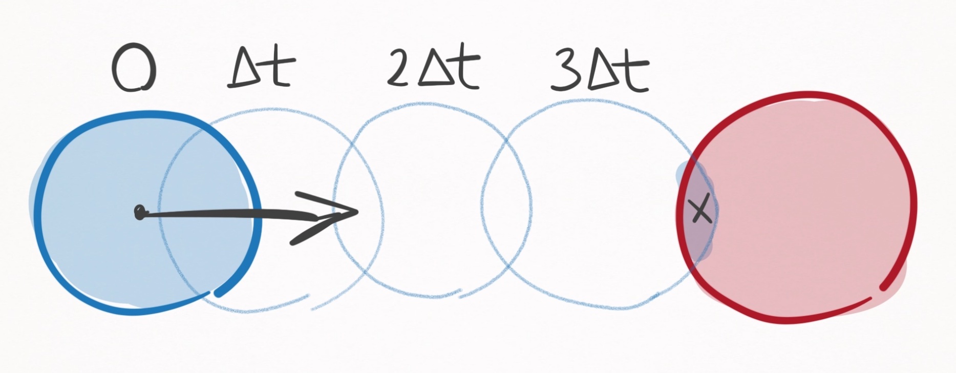Figure 1. Collision detection using discrete time evolution. The collision is detected at the timestep when the 2 balls overlap slightly (marked as x).

In the above scenario, the blue ball gets incrementally closer to the red ball with each timestep. Upon the third time step, the blue and red balls overlap slightly, triggering the detection of a collision. Herein lies the fundamental problem with discrete time evolution: collision events are never predicted, but rather detected after they were already supposed to have happened. So in the above example, the calculated collision time is $3 \Delta t$, even though the actual collision time is less than that–more like $2.8 \Delta t$.

The inaccuracy introduced by discrete time evolution can always be ameliorated by making $\Delta t$ smaller and smaller, yet there will always exist a margin of error on the order of $\Delta t$.

Furthermore, decreasing $\Delta t$ comes at massive computational cost. For example if you decrease the timestep 100-fold—sure, you increase the accuracy 100-fold—but you also increase the computational complexity 100-fold, since now you’ve gotta step through 100 times more time steps.

This can become brutal when dealing with pool simulations. Ball speeds commonly reach up to $10$ m/s, and a reasonable requirement for realism is that 2 balls should never intersect more than $1/100$th of a ball radius ($0.3$ mm). The required timestep for this level of realism is then $30$ microseconds. If the time from the cue strike to the last ball rolling is 10 seconds, that is $30,000$ time steps in total for one shot. If the level of realism is $1/1000$th a ball radius, that is $300,000$ time steps. Yikes.

The problem with this is all of the wasted computation… I don’t need $30$ microsecond time steps when all of the balls are far apart and barely moving. It is only really in select scenarios, such as a pool break, that realism demands such miniscule time steps.

To save computation, a smart discrete time evolution scheme would cut down on the number of time steps by making them adaptive depending on the state of the system. There are an infinite number of ways you could develop heuristics for an adaptive time stepper, that may be based on the distances between balls (if they are far apart, increase the time step), or based on velocities (if they are moving fast, decrease the time step). I’m not even going to go there because the possibilities are endless.

Continuous event-based evolution

The continuous event-based evolution algorithm was first developed by Leckie and Greenspan in a seminal paper entitled An Event-Based Pool Physics Simulator. If you would like to hear it straight from the horse’s mouth, a free pre-print of this publication is available here.

In the last post I presented a bunch of analytical equations of motion for ball trajectories, depending on whether the ball is stationary, spinning, rolling, sliding, or airborne.

These equations are perfect, because we can use them to evolve the ball states to any arbitrary time. The only (vital) problem is that events such as the collision in Figure 1 disrupt their validity, since they are developed assuming the ball acts in isolation.

For example, a ball rolling with a very high velocity may be destined to travel 50m in an isolated environment, yet collides with a cushion after just a few meters. Thus, the ball can safely be evolved via the rolling equations of motion up until the moment of collision, at which point the event must be resolved via the ball-cushion interaction equations. After the collision is resolved, the ball can be safely evolved up until the next event.

At this point, my mind was made up. I was going to use the continuous event-based algorithm for its speed and accuracy.

The algorithm, in its entirety

The rest of this post is concerned with detailing each and every aspect of this algorithm.

(1) Bird’s eye view

The prescription of evolving the equations of motion up until the next event forms the basis of the continuous event-based evolution algorithm. Simply stated, the algorithm goes like this:

Let’s walk through a loop of the algorithm. Assume the time is currently $t$, such that the system state is $S(t)$.

The first step is determining when the next event occurs. By next event, I mean that no other event precedes it. Assume this occurs an amount of time $\Delta t_E$ from the current time. Calculating $\Delta t_E$ is non-trivial, and my guess is that around 95% of the algorithm’s computational complexity is allocated to this specific task. The intricacies of this process will be described ad nauseam in the next section, but until then, assume $\Delta t_E$ is calculable.

Once calculated, the next step is to advance the system state from $S(t)$ to $S(t + \Delta t_E)$. This means updating each ball’s state to $s_i(t + \Delta t_E)$, where the equations of motion are determined depending on whether the ball is stationary, spinning, rolling, sliding, or airborne. Since we know that no other event occurs before $\Delta t_E$, we can safely evolve their equations to $t + \Delta t_E$, but no further.

Then, the states of any balls involved in the event must be resolved. Some examples: If the event is two balls colliding, their states are resolved via the ball-ball interaction equations. If the event is a ball contacting a cushion, its state is resolved via the ball-cushion interaction equations. If the event is a ball transitioning from sliding to rolling, its state is resolved by updating its equations of motions from sliding to rolling.

Once the states of the balls involved in the event have been solved, every ball now has equations of motion that will be valid until the next event occurs. Thus, the process repeats itself.

So that’s how the algorithm works, and it is superior to the discrete time evolution algorithm because one can advance directly to the next event. A typical shot may only have as little as 5 events, and calculating when they occur is orders of magnitude less computation than the hundreds of thousands of time steps used in discrete time evolution for a typical shot. Not to mention the only error in the continuous event-based evolution algorithm is due to floating point precision.

This is a beautifully simple algorithm, but its utterly useless if we can’t calculate $\Delta t_E$, the time until the next event–and that’s no easy task. That’s what I tackle in the next sections. First, I formally define what an event is and outline all possible events. Then, I define the strategy and in excruciating detail outline how to calculate the time until the next event.

(2) What are events?

In the context of the continuous event-based evolution algorithm, an event is defined as anything that invalidates the equations of motion for 1 or more balls, due to something that is unaccounted for in the equations of motion, such as a collision with another ball. In total, there are 8 events, 4 of which are collisions, 4 of which are transitions. I discuss each below.

ball-ball collision

Unlike every other event, the ball-ball collision involves 2 balls, one of which must be in a translating motion state: rolling, sliding, or airborne. The other ball may be in any motion state: stationary, spinning, rolling, sliding or airborne. The collision is governed by the ball-ball interaction equations.

Figure 2. The possible inputs and outputs of the ball-ball collision event.

If the incoming motion state isn’t airborne, then neither will be the outgoing state. Conversely, if the incoming motion state is airborne, so will be the outgoing motion state. In other words, a table-bound ball cannot become airborne due to a ball-ball collision. I admit this might be confusing if you consider what happens when an airborne ball collides with a ball on the table:

They both end up airborne. Since the line of centers between the two balls is directed into the table, the outgoing velocity of the table-bound ball has a component into the table, which initiates a ball-slate collision. Consequently, the table-bound ball (the 3-ball) becomes airborne. In the continuous event-based algorithm I’ve developed, the ball becomes airborne due to the ball-slate collision, not the ball-ball collision, which are separated by an infinitesimally small amount of time. As a network, the totality of this process looks like this:

Figure 3. Network representation of events and ball motion states for the ball-ball collision slow-mo video.

ball-cushion collision

The ball-cushion collision involves just one ball, which must be in a translating motion state: rolling, sliding, or airborne. The output state is either sliding or airborne. The collision is governed by the ball-cushion interaction equations.

Figure 4. The possible inputs and outputs of the ball-cushion collision event.

The only way to have an outgoing airborne motion state is if the incoming motion state is also airborne. Just like in the ball-ball collision, you may find this confusing, since after a collision with a cushion, you often see it airborne:

Yet just like as described in the ball-ball collision, the ball becomes airborne due to the ball-slate collision, which occurs an infinitesimally small amount of time after the ball-cushion collision. You can see the above shot represented as an interaction:

Figure 5. Network representation of events and ball motion states for the ball-cushion slow-mo video

ball-slate collision

The ball-slate collision occurs when a ball contacts the table with a velocity component into the table ($-z-$direction). The collision is governed by the ball-slate interaction equations.

Stationary, spinning, and rolling balls necessarily have 0 speed along the $z-$axis, so the only available input motion states are sliding and airborne.

So when do we see ball-slate collisions? An airborne ball undergoes a ball-slate collision whenever it contacts the table. Additionally, we’ve seen in Figures 3 and 5 that sliding balls can also have non-zero velocities in the $z-$direction (caused by ball-ball and ball-cushion collisions that immediately precede the ball-slate collision), and also undergo ball-slate collisions.

The first possible outgoing motion state of the ball-slate interaction is being airborne. The second possible outgoing motion state is sliding, which occurs when the ball doesn’t have enough velocity to become airborne.

Figure 6. The possible inputs and outputs of the ball-slate collision event.

ball-pocket collision

Of all the events, this is definitely the most fabricated. You may hear ball-pocket collision and think about all the complexities of the ball leaving the slate and falling into the pocket, bouncing off the sides of the pocket, etc. but that’s not what I mean by ball-pocket collision. In fact, I don’t really plan to model that.

Instead, the ball-pocket collision is merely a way to determine if a ball is pocketed and if it is, removing it from the simulation. Basically, if a ball undergoes a ball-pocket collision, the ball is considered pocketed. It went in the hole. Good job.

To resolve the collision, the ball is simply removed from the simulation.

transition events

In Figures 2-6, I’ve shown that collisions often induce motion state transitions, however in each of those cases the transition is caused by the collision. Yet motion state transitions also occur naturally:

In the above short clip, the ball transitions from spinning to stationary. This is considered an event, because upon becoming stationary, the ball’s equations of motion (spinning) become invalid and need to be updated to the stationary equations of motion.

As a matter of interest, if the equation was not updated, it dictates that the ball would begin spinning in the reverse direction, gaining more and more rotational kinetic energy indefinitely. This is obviously non-physical, and illustrates the need to properly handle motion state transition events.

Mathematically, there are $5^4 = 1024$ transitions, but only 4 occur naturally. Thus there are only 4 transition events:

1. spinning-stationary
2. rolling-stationary
3. rolling-spinning
4. sliding-rolling

Fundamentally, these transitions happen due to a loss of energy due to friction. So these transitions are always from high energy to low energy.

I’ve actually omitted 2 very rare transition events. In theory, a ball can transition from sliding to stationary if the perfect amount of backspin is applied. Same goes for sliding to spinning. So technically, there are 2 more transition events:

5. sliding-stationary (very rare)

6. sliding-spinning (very rare)

Yet, there is 0 margin for error for these scenarios. In virtually all simulated cases, a ball will exit the sliding state with non-zero speed (using 64-bit floats with SI units yields femtometer $(10^{-15})$ per second precisions). For this reason, the sliding-stationary and sliding-spinning transition events can in all practical senses be decomposed into 2 transition events separated by some very small amount of time. For example, the sliding-stationary transition can be decomposed into the sliding-rolling transition followed by a rolling-stationary transition.

Figure 8. The sliding-stationary transition event can be decomposed into the sliding-rolling followed by the rolling-stationary transition events.

This wraps up my description of the possible event types.

(3) The strategy

We now know all the possible types of events. So what’s the strategy for calculating when the next event occurs? As it turns out, the most feasible strategy is to explicitly calculate the time until every possible next event. If you calculate the time until literally every possible next event, then by definition the one that occurs in the shortest amount of time is the one that physically occurs next.

Toy example

Consider the example pictured in Figure 9. Ball A is sliding, balls B & C are stationary, and there are no other balls on the table. For simplicity, assume there are no cushions or pockets and that the table surface extends indefinitely. To calculate the next event, we need to consider all possible events. So let’s do that.

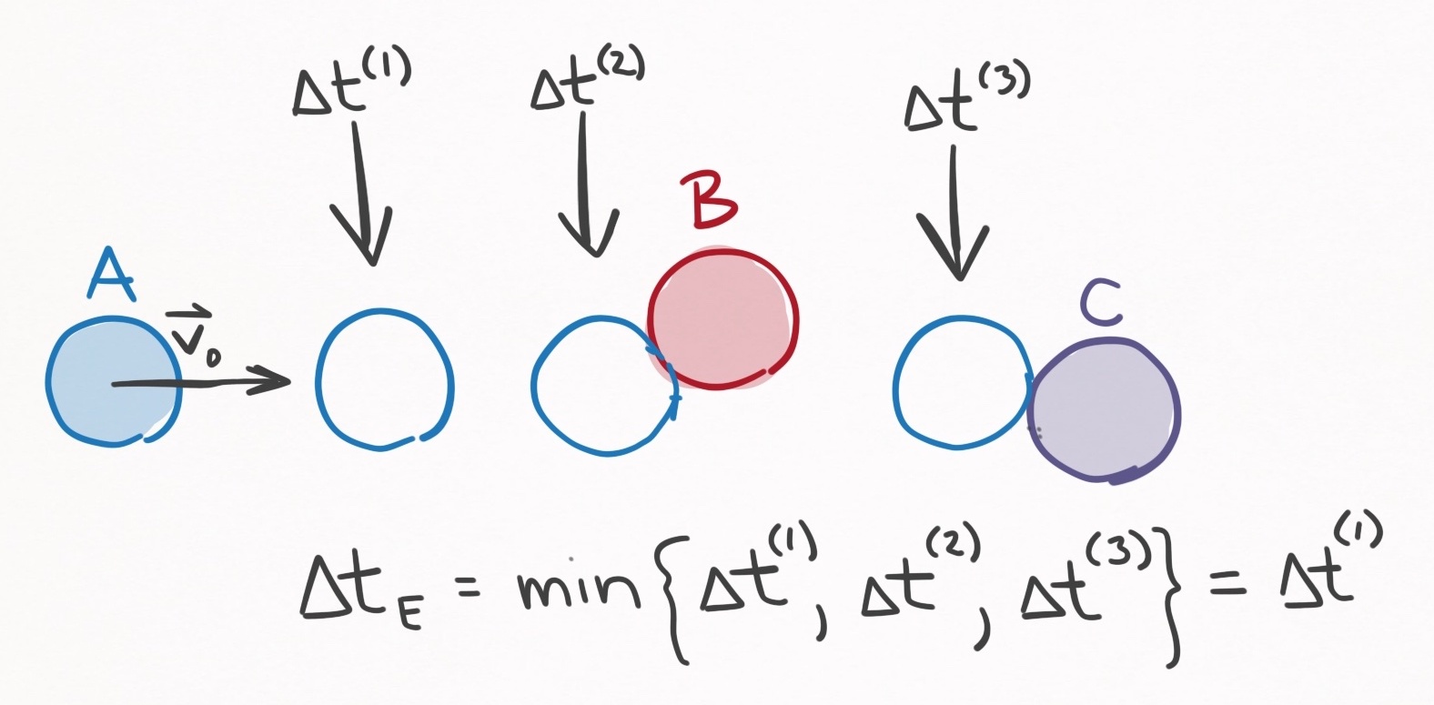Figure 9. A system with 1 sliding ball (A) and 2 stationary balls (B & C). The solid-filled balls indicate where the balls currently are. There are 3 next events: (1) Ball A can transition from sliding to rolling $(\Delta t^{(1)})$, (2) ball A can collide with ball B $(\Delta t^{(2)})$, or (3) ball A can collide with ball C $(\Delta t^{(3)})$.

• ball-cushion collision events. Since there are no cushions, there are no ball-cushion collision events to consider.
• ball-pocket collision events. Let’s also assume there are no pockets, so no ball-pocket collision events to consider either.
• ball-slate collision events. Balls B and C are stationary, so cannot undergo a ball-slate collision event. If ball A has a velocity component into the table, then the next event would be a ball-slate collision, since it would occur at $t=0$. But for the sake of example, let’s assume ball A has no velocity component into the table. Then there are no ball-slate collision events to consider.
• ball-ball collision events. There are 3 potential ball-ball collision events: between balls A & B, A & C, and B & C. However, since 2 stationary balls cannot collide, the B & C collision is an impossible event, and only A & B, and A & C collisions need to be considered.
• transition events. Since balls B and C are stationary, there are no available transition events–they are already in their lowest energy states. On the other hand, Ball A is sliding, so a sliding-rolling transition event is a possibility for Ball A.

In summary, there are 3 events to consider: (1) a sliding-rolling transition for ball A, (2) a ball-ball collision with balls A and B, and (3) a ball-ball collision with ball A and C.

Based on how I’ve drawn Figure 9, it’s obvious that the next event is the sliding-rolling transition, yet in general the time for each of these events must be calculated explicitly. If ball A was spinning a lot, ball A could collide with ball B whilst spinning, which would make the collision with ball B the next event. In fact, we can’t even rule out that a collision with C is not the next event, which could happen if ball A has a curved trajectory that goes around ball B.

So the point is this: given a system state $S(t)$, the only way to determine the next event $\Delta t_E$, is to explicitly calculate the time until all possible next events. The next event is the one that occurs in the smallest amount of time.

This means we must develop means to calculate the time until every possible next event, which is the subject of the next section. Buckle your seatbelts.

(4) Calculating possible event times

Transition times

Transition times are the easiest to calculate, so I’ll start with them.

The spinning-stationary transition is defined by the moment at which a spinning ball reaches 0 angular velocity in the $z-$direction. From the spinning equations of motion, the angular velocity as a function of time is given by

\[\omega_z(t) = \omega_{0z} - \frac{5\mu_{sp}g}{2R}t \notag\]

Setting this to 0 and solving for time yields the spinning-stationary transition time:

Reminder, this equation is significant because for a given time $t$, the spinning-stationary event for every spinning ball must be considered as a potential next event.

On to the next. Both the rolling-stationary events and the rolling-spinning events are defined by the moment at which a ball’s center of mass velocity reaches 0. From the rolling equations of motion, the velocity of a rolling ball as a function of time is given by

\[\vec{v}(t) = \vec{v}_0 - \mu_r g t \hat{v}_0 \label{rolling_velocity} \notag\]

Taking the magnitude of both sides, setting the LHS to 0, and solving for time yields the rolling-stationary and rolling-spinning transition times:

Reminder, this equation is significant because for a given time $t$, the rolling-spinning and rolling-stationary transition events for every rolling ball must be considered as a potential next event.

Finally, we got the sliding-rolling transition, which is defined by the moment at which the relative velocity $\vec{u}$ becomes $\vec{0}$. From the sliding equations of motion, the relative velocity as a function of time is given by

\[\vec{u}(t) = (u_0 - \frac{7}{2} \mu_s g t ) \, \hat{u}_0 \notag\]

Taking the magnitude of both sides, setting the LHS to 0, and solving for time yields the sliding-rolling transition time:

Reminder, this equation is significant because for a given time $t$, the sliding-rolling transition event for every sliding ball must be considered as a potential next event.

That’s all of the event transition times. Short and sweet.

Ball-ball collision times

We are on the search for calculating all possible next events.

A very large subcategory of next possible events is all of the ball-ball collisions that may occur. In fact, if there are 15 balls on the table, there are $_ {15}\text{C} _ {2} = 105$ different ball-ball collision events that may be the next event, and the time until each of them must be explicitly calculated. As we will see, many may take an infinite or non-real amount of time.

First, an important assumption needs to be discussed. Suppose the current time is $t$, and you want to calculate the time until collision, $\Delta t_E$, between two balls with states $s^{(i)}(t)$ and $s^{(j)}(t)$. I’ll call this the $i-j$ collision event. Within the time range $[t, t + \Delta t_E]$, I will assume neither of the balls are involved in any other event. This means neither of the 2 balls engage in any transitions or collisions. If either did, then the intervening event necessarily precedes the $i-j$ collision event, which means it doesn’t need to be considered as a candidate for the next event.

To predict when two balls colide, we need a collision condition. The collision occurs when the distance between the center of masses of the two balls is $2R$, where $R$ is the radii of the balls.

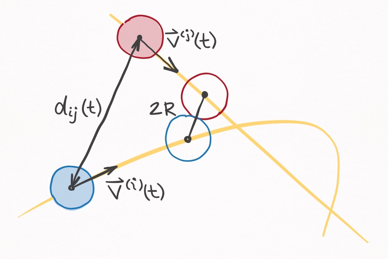Figure 10. On overhead view of a collision trajectory of the $i\text{th}$ and $j\text{th}$ balls. The magnitude of the distance vector is $d _{ij}(t)$, and the collision occurs when $d _{ij}$ is $2R$.

Mathematically, we can track the distance between the two balls as a function of time by defining a distance vector $\vec{d}_{ij}(t)$:

\[\vec{d}_{ij}(t) = \vec{r}^{(j)}(t) - \vec{r}^{(i)}(t) \label{dist_vec_defn}\]

where $\vec{r}^{(i)}(t)$ is the position of the $i\text{th}$ ball and $\vec{r}^{(j)}(t)$ is the position of the $j\text{th}$ ball. The collision condition is thus

\[\lvert \vec{d}_{ij}(\Delta t_E) \rvert = 2R \label{collision}\]

where $\Delta t_E$ is the collision time. The forms of $\vec{r}^{(i)}(t)$ and $\vec{r}^{(j)}(t)$ will depend on the whether the balls are stationary, spinning, rolling, spinning, or airborne. Fortunately, we have equations of motion for each of these scenarios, each of which can be cast in the following form:

\[\vec{r}^{(i)}(t) = \begin{bmatrix} a_x^{(i)} t^2 + b_x^{(i)} t + c_x^{(i)} \\ a_y^{(i)} t^2 + b_y^{(i)} t + c_y^{(i)} \\ a_z^{(i)} t^2 + b_z^{(i)} t + c_z^{(i)} \end{bmatrix} \label{quad_r}\]

As you can see, each component can be expressed as a quadratic equation with respect to time (though in many cases the $a$, $b$, and $c$ coefficients are 0). The coefficients depend on which motion state the ball is in. For example, Eq. $\eqref{quad_r}$ for a rolling ball has the following coefficients:

\[a_x^{(i)} = - \frac{1}{2} \mu_r g \cos(\phi^{(i)}) \notag\] \[a_y^{(i)} = - \frac{1}{2} \mu_r g \sin(\phi^{(i)}) \notag\] \[a_z^{(i)} = 0 \notag\] \[b_x^{(i)} = v_0^{(i)} \cos(\phi^{(i)}) \notag\] \[b_y^{(i)} = v_0^{(i)} \sin(\phi^{(i)}) \notag\] \[b_z^{(i)} = 0 \notag\] \[c_x^{(i)} = r_{0x}^{(i)} \notag\] \[c_y^{(i)} = r_{0y}^{(i)} \notag\] \[c_z^{(i)} = 0 \notag\]

which was determined by looking at the the rolling equations of motion. As another example, looking at the stationary equations of motion reveals that a stationary ball has the following coefficients in Eq. $\eqref{quad_r}$:

\[a_x^{(j)} = a_y^{(j)} = a_z^{(j)} = 0 \notag\] \[b_x^{(j)} = b_y^{(j)} = b_z^{(j)} = 0 \notag\] \[c_x^{(j)} = r_{0x}^{(j)} \notag\] \[c_y^{(j)} = r_{0y}^{(j)} \notag\] \[c_z^{(j)} = 0 \notag\]

Regardless of the particulars, the critical point is that a ball’s trajectory is defined by these 9 coefficients. To determine if two balls collide, we can formulate the distance vector $\vec{d}(t)$ from Eq. $\eqref{dist_vec_defn}$ in terms of these 18 coefficients (2 balls, 9 coefficients each):

\[\vec{d}_{ij}(t) = \begin{bmatrix} A_x t^2 + B_x t + C_x \\ A_y t^2 + B_y t + C_y \\ A_z t^2 + B_z t + C_z \\ \end{bmatrix} \label{diff_vec}\]

where

\[A_x = a_x^{(j)} - a_x^{(i)} \label{A_x_ball}\] \[A_y = a_y^{(j)} - a_y^{(i)} \label{A_y_ball}\] \[A_z = a_z^{(j)} - a_z^{(i)} \label{A_z_ball}\] \[B_x = b_x^{(j)} - b_x^{(i)} \label{B_x_ball}\] \[B_y = b_y^{(j)} - b_y^{(i)} \label{B_y_ball}\] \[B_z = b_z^{(j)} - b_z^{(i)} \label{B_z_ball}\] \[C_x = c_x^{(j)} - c_x^{(i)} \label{C_x_ball}\] \[C_y = c_y^{(j)} - c_y^{(i)} \label{C_y_ball}\] \[C_z = c_z^{(j)} - c_z^{(i)} \label{C_z_ball}\]

Plugging Eq. $\eqref{diff_vec}$ into the collision condition Eq. $\eqref{collision}$ yields an equation whose roots describe the time until two arbitrarily balls collide:

Eq. $\eqref{ball_poly}$ can be solved analytically or numerically to reveal if/when the $i-j$ collision event occurs. This prescription can be applied for each ball-ball pair.

Ball-cushion collision times

Another subset of possible events are all of the ball-cushion collisions—and there are a lot of collisions to account for.

In my model, I deconstruct the entire cushion contact surface into a collection of straight-line cushion segments, and potential collisions for each ball must be assessed for every cushion segment. On a standard table with 6 pockets, there are 18 cushion segments (Figure 11). With 15 balls on the table, that is 270 potential ball-cushion collision events that must be explicitly considered as the next event.

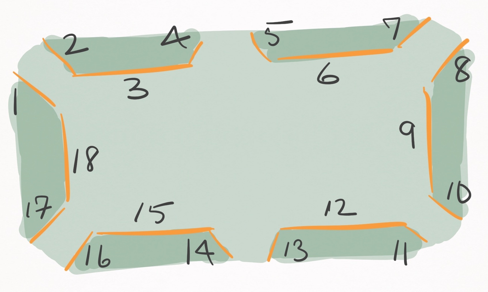
Figure 11. On a standard table with 6 pockets, there are 18 straight-line segments that define the cushion contact surfaces.

Overall, the treatment is very similar to the ball-ball collision time calculation: develop an expression for the distance between the ball and the cushion as a function of time–based off the quadratic form of the ball’s trajectory–and solve for the collision condition. I do this two ways, one which is simple, and one which is very, very, very ugly but more accurate.

The first is simpler, and defines the ball-cushion collision as the moment the ball contacts a plane that extends vertically from the cushion segment’s edge. I call this the collision plane.

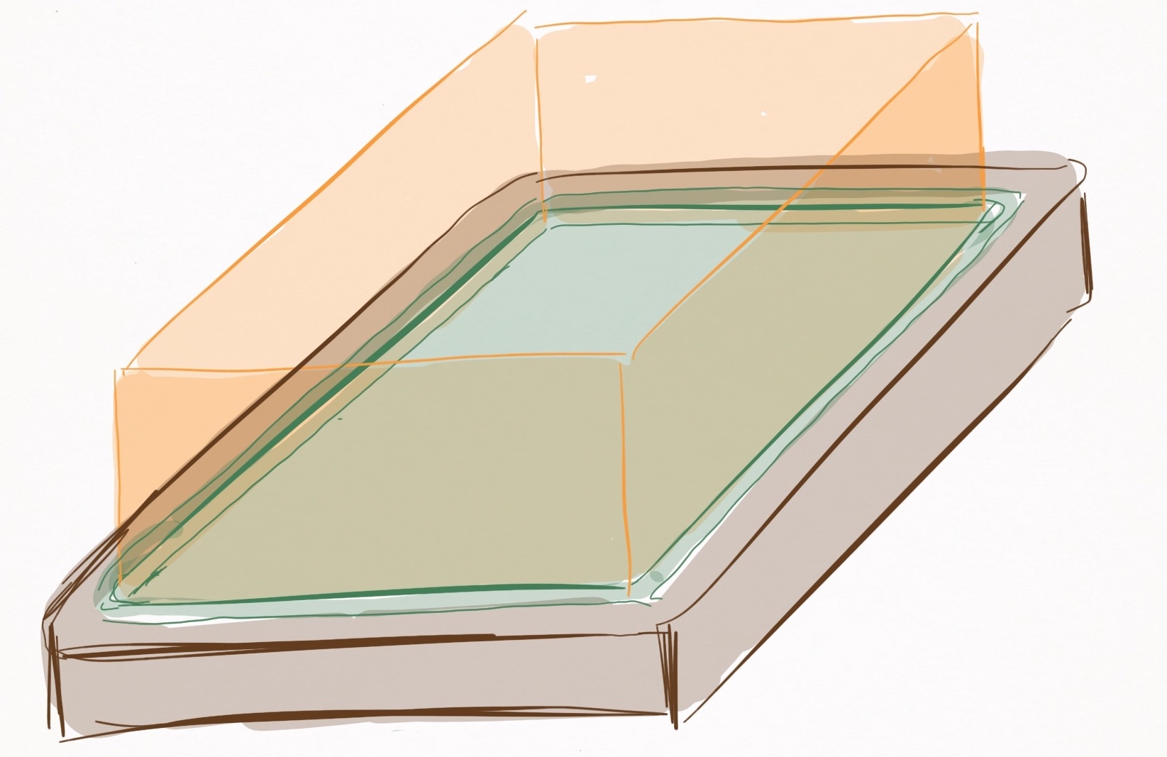
Figure 12. Visualization of collision planes (orange) that extend vertically from the cushion edges. The planes extend infinitely in the vertical direction (despite how they are pictured). A ball-cushion collision is assumed to occur whenever a ball contacts a collision plane.

This assumption is convenient and mostly accurate when balls remain on or nearly on the table, but creates false-positive collision events when balls in airborne motion states intersect the collision plane. Even if balls remain on or nearly on the table, there is a slight inaccuracy introduced that depends on how airborne the ball is, which is depicted in Figure 13. Nevertheless, convenience often outweighs accuracy.

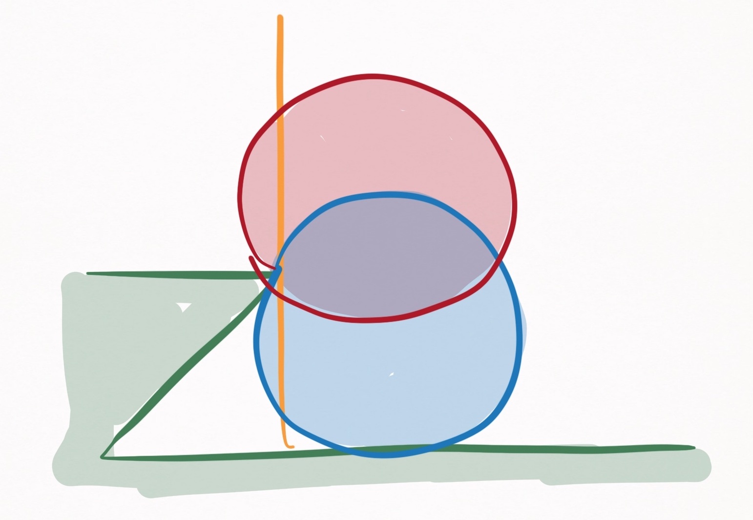
Figure 13. A side view of the collision plane (orange). Two mock balls (red & blue) are pictured at the moment they contact the cushion edge. As seen, there is a discrepancy between when balls contact the collision plane versus the cushion edge.

The collision condition for a collision of the $i\text{th}$ ball with the $j\text{th}$ cushion segment occurs when the $i\text{th}$ ball contacts the $j\text{th}$ cushion segment’s collision plane. The most convenient way to define the collision plane is with two points on the $xy-$plane, which can be expressed as these two vectors:

\[\vec{p}_1^{(j)} = \langle p_{1x}^{(j)}, \, p_{1y}^{(j)}, \, 0 \rangle \label{p1_plane}\] \[\vec{p}_2^{(j)} = \langle p_{2x}^{(j)}, \, p_{2y}^{(j)}, \, 0 \rangle \label{p2_plane}\]

The collision plane is the plane that extends vertically from the line connecting $\vec{p}_1^{(j)}$ and $\vec{p}_2^{(j)}$. We can also define the collision plane as a classic $y = m x + b$ scenario by using these points:

\[y = m x + b \notag\]

Channel your high school math education to express $m$ and $b$ in terms of the points:

\[y = \frac{p_{2y}^{(j)} - p_{1y}^{(j)}}{p_{2x}^{(j)} - p_{1x}^{(j)}} x + p_{1y}^{(j)} - \frac{p_{2y}^{(j)} - p_{1y}^{(j)}}{p_{2x}^{(j)} - p_{1x}^{(j)}} p_{1x}^{(j)} \notag\]

Finally, cast everything onto the left-hand side:

\[l_x^{(j)} x + l_y^{(j)} y + l_0^{(j)} = 0 \notag\]

where

\[l_x^{(j)} = -\frac{p_{2y}^{(j)} - p_{1y}^{(j)}}{p_{2x}^{(j)} - p_{1x}^{(j)}} \\ l_y^{(j)} = 1 \\ l_0^{(j)} = \frac{p_{2y}^{(j)} - p_{1y}^{(j)}}{p_{2x}^{(j)} - p_{1x}^{(j)}} p_{1x}^{(j)} - p_{1y}^{(j)} \label{ls}\]

Alright, the shortest distance between a point $(p_x, p_y, p_z)$ and the collision plane is defined by

\[d = \frac{\lvert l_x^{(j)} p_x + l_y^{(j)} p_y + l_0^{(j)} \rvert}{\sqrt{l_x^{(j)\, 2} + l_y^{(j)\, 2}}} \label{dist_to_plane}\]

(Source)

This describes the distance between the point $(p_x, p_y, p_z)$ and a plane that extends infinitely in the $xy-$plane, rather than a plane that terminates at the points $\vec{p}_1^{(j)}$ and $\vec{p}_2^{(j)}$. We will have to deal with this oversight in a minute.

Rather than use an arbitrary point $(p_x, p_y, p_z)$, here I throw in the trajectory of the $i\text{th}$ ball from Eq. $\eqref{quad_r}$:

\[d_{ij}(t) = \frac{\lvert l_x^{(j)} r_x^{(i)}(t) + l_y^{(j)} r_y^{(i)}(t) + l_0^{(j)} \rvert}{\sqrt{l_x^{(j)\, 2} + l_y^{(j)\, 2}}} \notag\] \[d_{ij}(t) = \frac{\lvert l_x^{(j)} (a_x^{(i)} t^2 + b_x^{(i)} t + c_x^{(i)}) + l_y^{(j)} (a_y^{(i)} t^2 + b_y^{(i)} t + c_y^{(i)}) + l_0^{(j)} \rvert}{\sqrt{l_x^{(j)\, 2} + l_y^{(j)\, 2}}} \notag\]

where $d_{ij}$ is the distance between the $i\text{th}$ ball and the $j\text{th}$ cushion segment.

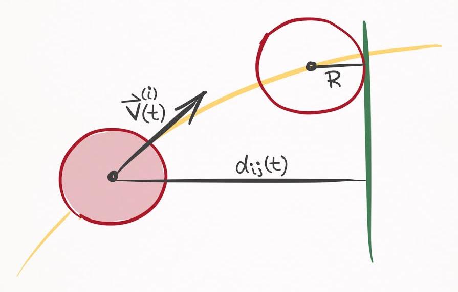
Figure 14. A top down view of a collision trajectory of the $i\text{th}$ ball with the $j\text{th}$ cushion segment. The magnitude of the distance vector is $d _{ij}(t)$, and the collision occurs when $d _{ij}$ is $R$–in other words when the ball contacts the collision plane (green line).

With an expression that describes the distance between the $i\text{th}$ ball and the $j\text{th}$ cushion segment, I can mathematically express the collision condition by setting $d_{ij}$ to $R$, which by definition happens at a time $\Delta t_E$:

\[\lvert l_x^{(j)} (a_x^{(i)} \Delta t_E^2 + b_x^{(i)} \Delta t_E + c_x^{(i)}) + l_y^{(j)} (a_y^{(i)} \Delta t_E^2 + b_y^{(i)} \Delta t_E + c_y^{(i)}) + l_0^{(j)} \rvert - \\ R\sqrt{l_x^{(j)\, 2} + l_y^{(j)\, 2}} = 0 \notag\]

So this is the collision condition, which is quadratic with respect to time. Calculating the roots of this quadratic will reveal if and when a collision occurs. Specifically, if there are any real, positive roots to the equation, a collision between the $i\text{th}$ ball and $j\text{th}$ cushion is a potential next event.

There is just one critical problem. This collision condition assumes the collision plane extends infinitely in the $xy-$plane, rather than terminating at the points $\vec{p}_1^{(j)}$ and $\vec{p}_2^{(j)}$, each which define the cushion segment’s physical boundaries. This is bad news, because there will be many false-positive collision events for a given cushion segment if this is not dealt with. Check out Figure 15.

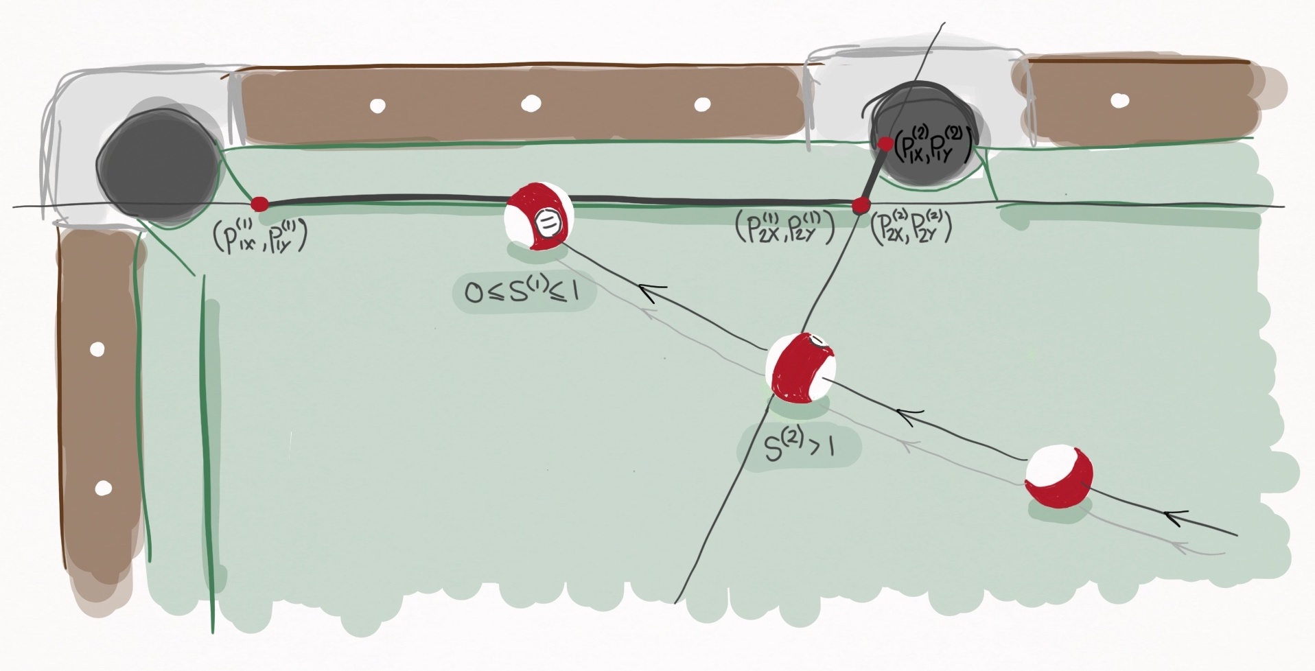
Figure 15. A ball transits the playing surface and encounters two potential cushion segments. The first cushion segment is defined by the points $(p _{1x}^{(1)}, p _{1y}^{(1)})$ and $(p _{2x}^{(1)}, p _{2y}^{(1)})$ and represents the long rail. The second cushion segment is defined by the points $(p _{1x}^{(2)}, p _{1y}^{(2)})$ and $(p _{2x}^{(2)}, p _{2y}^{(2)})$ and represents the left jaw of the side pocket. The ball’s collision with the first cushion segment is legitimate because $0 \le s^{(1)} \le 1$, whereas the collision with the second cushion segment is illegitimate because $s^{(2)} > 1$.

The collision plane of cushion segment 2 defines the left jaw of the side pocket. It begins at $(p _{1x}^{(2)}, p _{1y}^{(2)})$ and ends at $(p _{2x}^{(2)}, p _{2y}^{(2)})$. But because of Eq. $\eqref{dist_to_plane}$’s flawed assumption, the collision plane mathematically extends into the playing surface, and triggers false collision events with unsuspecting passersby, e.g. the 11-ball.

Obviously this won’t do. Fortunately, the solution is self-apparent: if the alleged collision occurs outside the boundary defined by the physical portion of the collision plane, disregard it. I needed to express this mathematically, and I did it by parameterizing a cushion segment’s collision plane with the following representation:

\[\vec{p}^{(j)} = \begin{bmatrix} p_{1x}^{(j)} + (p_{2x}^{(j)} - p_{1x}^{(j)}) \, s \\ p_{1y}^{(j)} + (p_{2y}^{(j)} - p_{1y}^{(j)}) \, s \\ z \end{bmatrix} \label{parameterized_plane}\]

Since it is a vertical plane, $z$ is a free parameter

$s$ is the parameter that defines where on the plane you lie. It’s basically a slider scale that goes from $-\infty$ to $+\infty$. But very importantly, this parameterization is defined such that $s=0$ corresponds to the coordinate $\langle p_{1x}^{(j)}, p_{1y}^{(j)}, z \rangle$ and $s=1$ corresponds to the coordinate $\langle p_{2x}^{(j)}, p_{2y}^{(j)}, z \rangle$. In other words, the range $s \in [0, 1]$ defines the physical portion of the collision plane!

So to see whether or not any collision predicted by the collision condition is legitimate, we need only find the $s$ value at the time of collision. If $0 \le s \le 1$, the collision is legitimate, and otherwise it is not and can be ignored.

According to Eq. 3 of this source, the value of $s$ at the collision time can be calculated via the following equation:

\[s = - \frac{ (\vec{p}_1^{(j)} - \vec{r}^{(i)}(t + \Delta t_E)) \bullet (\vec{p}_2^{(j)} - \vec{p}_1^{(j)}) }{ (\vec{p}_2^{(j)} - \vec{p}_1^{(j)}) \bullet (\vec{p}_2^{(j)} - \vec{p}_1^{(j)}) } \label{s_at_plane}\]

Now we are fully equipped to detect ball-cushion collisions.

---

As a more advanced treatment, I now consider a more physically accurate case in which the cushion segment is treated as a line that coincides with the cushion segment’s edge, depicted in orange in Figure 16.

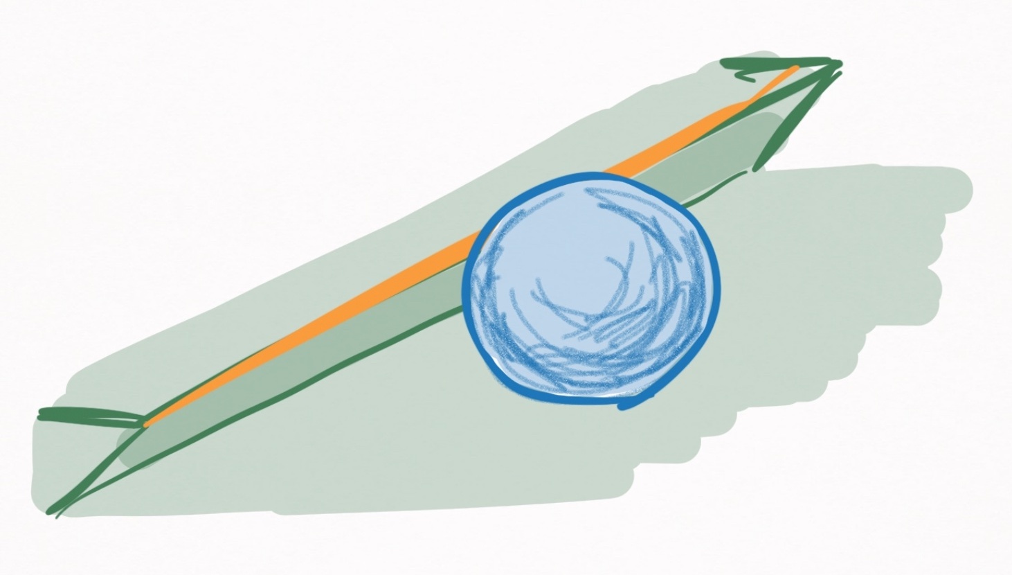
Figure 16. A ball in contact with a cushion. Mathematically, the ball-cushion collision is detected by defining the cushion’s edge, highlighted in orange.

Defining a collision line rather than a collision plane allows complete accuracy in determining collision times and permits balls to fly off the table, thereby avoiding all false-positive ball-cushion collision events that occur with a collision plane.

The most convenient way to define the collision line of a cushion segment is to specify two points, where the line connecting them is the collision line. The points for the collision line of the $j\text{th}$ cushion segment can be defined with the following vectors

\[\vec{p}_1^{(j)} = \langle p_{1x}^{(j)}, \, p_{1y}^{(j)}, \, h \rangle \label{p1_line}\] \[\vec{p}_2^{(j)} = \langle p_{2x}^{(j)}, \, p_{2y}^{(j)}, \, h \rangle \label{p2_line}\]

This time the $z-$component is not free, but rather fixed at the height of the cushion, $h$. Here I assume $h$ is constant, but it may be fun exploring a relaxation of this assumption later. With these 2 vectors defined, the line can be parameterized via the following vector:

\[\vec{p}^{(j)} = \begin{bmatrix} p_{1x}^{(j)} + (p_{2x}^{(j)} - p_{1x}^{(j)}) \, s\\ p_{1y}^{(j)} + (p_{2y}^{(j)} - p_{1y}^{(j)}) \, s\\ h \end{bmatrix} \label{p1_vec}\]

where $s$ determines where on the line you are.

Just as the distance of a point to the collision plane is given by Eq. $\eqref{dist_to_plane}$, we need an equation for the distance of a point to the collision line.

If such a point is described by the vector $\vec{p}_0 = \langle p _{0x}, p _{0y}, p _{0z} \rangle$, then the minimum distance to the collision line is

\[d = \frac{\lvert (\vec{p}_0 - \vec{p}_1^{(j)}) \times (\vec{p}_0 - \vec{p}_2^{(j)}) \rvert} {\lvert \vec{p}_2^{(j)} - \vec{p}_1^{(j)} \vert} \notag\]

(Source) where $\times$ denotes the cross product. By replacing $\vec{p}_0$ with the trajectory of the $i\text{th}$ ball, we get the distance of the $i\text{th}$ ball to the $j\text{th}$ cushion segment as a function of time.

\[d_{ij}(t) = \frac{\lvert (\vec{r}^{(i)}(t) - \vec{p}_1^{(j)}) \times (\vec{r}^{(i)}(t) - \vec{p}_2^{(j)}) \rvert} {\lvert \vec{p}_2^{(j)} - \vec{p}_1^{(j)} \vert} \label{dist_to_line}\]

Like before, the collision condition is defined by setting $d_{ij}$ to $R$, which by definition happens at time $\Delta t_E$. After substituting Eq. $\eqref{quad_r}$ into Eq. $\eqref{dist_to_line}$, the algebra blows up.

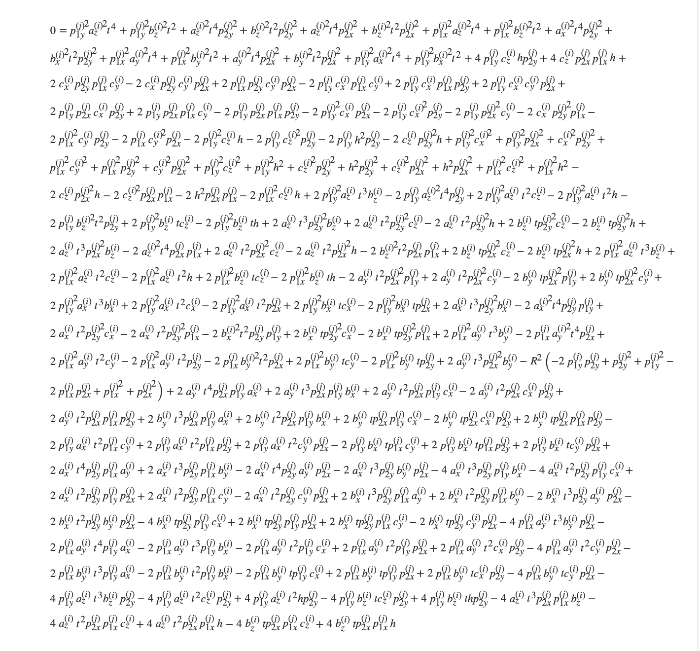
This page experiences a lot of lag if I try to render this math as an html object, so I took the above screenshot instead. Click here for the html version.

It’s beauty no doubt challenges that of Euler’s $e^{i\pi} + 1 = 0$. Whether or not you agree doesn’t take away from the fact that this is a legitimate quartic polynomial with respect to time, the roots of which describe the time until collision of ball $i$ and cushion segment $j$.

The only thing that needs to be done is grouping the different orders together so the solution can be presented.

Wow.

Ball-slate collision times

In comparison to the ball-cushion collision, this is a breeze.

The ball-slate collision occurs either when a sliding ball has a $-z-$velocity component, or an airborne ball hits the slate. The first case is somewhat pendantic, because if it has a $-z-$velocity component, the time until the ball-slate collision is by definition 0. So the real calculation is determining when an airborne ball hits the slate.

An airborne ball hits the slate when $r_z = R$, where $R$ is the ball’s radius. According to the airborne equations of motion, $r_z(t)$ is given by

\[r_z(t) = r_{0z} + v_{0z} t - \frac{1}{2} g t^2 \notag\]

Setting this to $R$ and solving for time yields the ball-slate collision time:

Reminder, this equation is significant because for a given time $t$, the ball-slate collision event for every sliding and airborne ball must be considered as a potential next event.

Ball-pocket collision times

So as mentioned, the ball-pocket collision exists as a means to determine when a ball is pocketed, and to remove the ball from the simulation when it is pocketed. Defining the ball-pocket collision condition requires a suitable geometry for pockets, which I am going to be very rudimentary about.

Basically, the $j\text{th}$ pocket is going to be a circle with center $(a^{(j)}, b^{(j)})$ and radius $R^{(j)}$. Here’s an illustration because I spoil you:

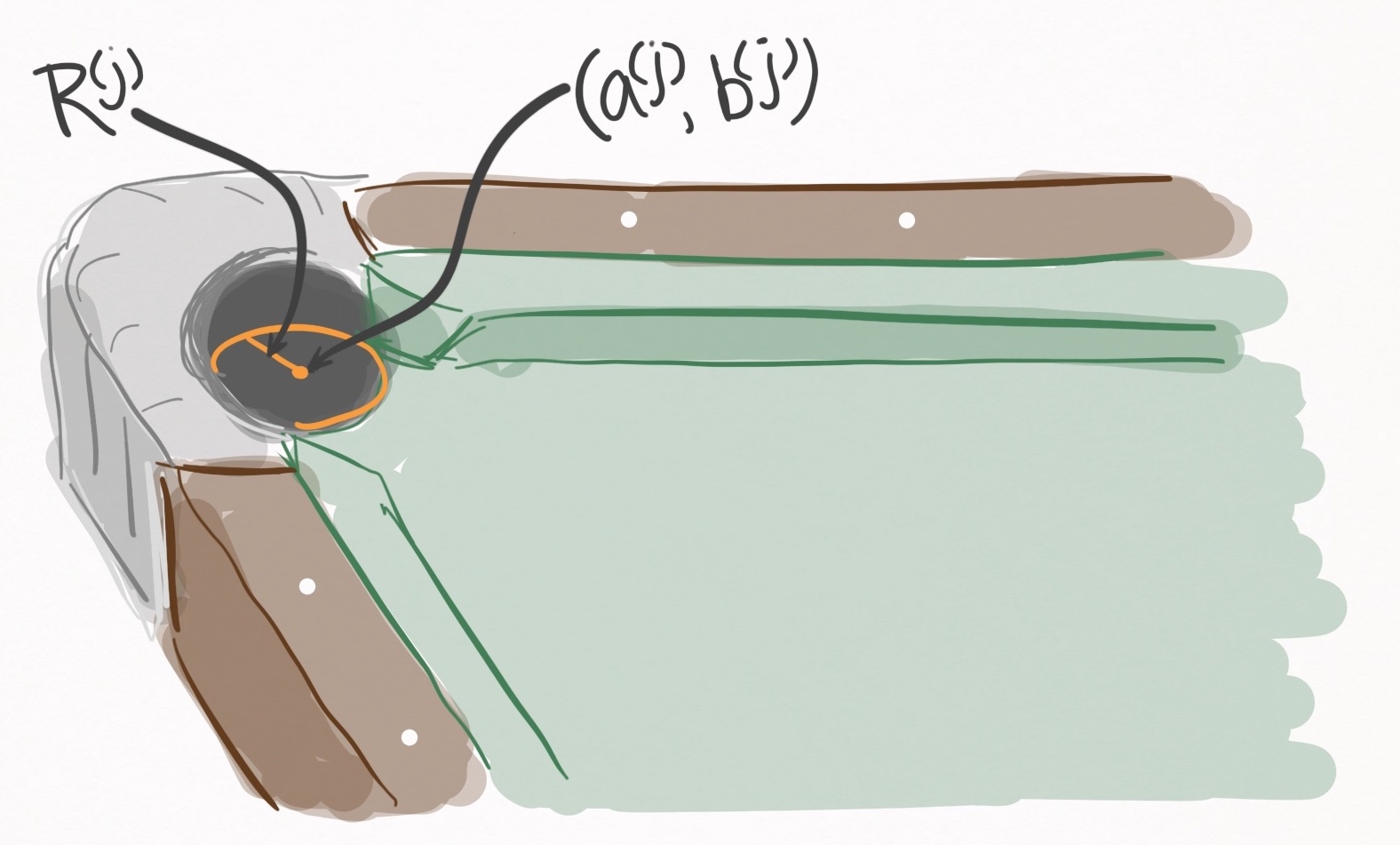
Figure 17. A depiction of the pocket geometry (shown in orange) for the $j\text{th}$ pocket. The center is $(a^{(j)}, b^{(j)})$ and the radius is $R^{(j)}$.

First of all, we are able to exclude any balls that are stationary, spinning, or airborne. So we are only including balls that are rolling or sliding. Excluding airborne balls simplifies things considerably, since we can assume that $r_z^{(i)}(t)$ has a constant value of $R$, and therefore we can treat the collision condition as a 2D problem.

Actually, I’d like to modify the above statement slightly. If you absolutely slam a ball into a pocket, it is likely to be slightly airborne, if only by a millimeter. Yet it still falls into the pocket because the back lip of the pocket is at a height higher than the ball’s radius, thus redirecting the ball into the pocket. Let’s call this lip height $h_M$ and assume that any ball with $r_z(t)$ less than $h_M$ is pocketed, and any ball greater than $h_M$ isn’t. An obviously crude means of modelling what in reality is a complex rigid body dynamics problem that doesn’t easily lend itself to continuous event-based evolution.

Based on my own table, it seems like a reasonable value for $h_M$ is $7R/5$.

To muster up a mathematical collision condition between the $i\text{th}$ ball and the $j\text{th}$ pocket, I define the distance between the ball and the center of the pocket:

\[d_{ij}(t) = \sqrt{(r_x^{(i)}(t) - a^{(j)})^2 + (r_y^{(i)}(t) - b^{(j)})^2} \notag\]

The collision is assumed to occur at the moment the ball rolls over the table’s edge:

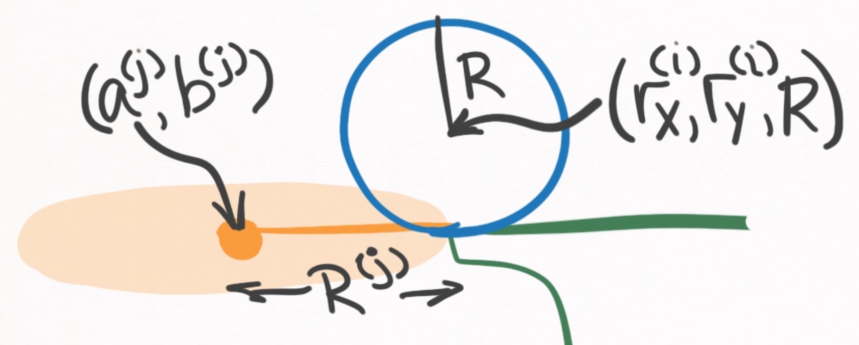
Figure 18. Side profile of a pocket and ball during the moment of the ball-pocket collision.

At this moment, $d_{ij}(\Delta t_E) = R^{(j)}$, where $R^{(j)}$ is the radius of the pocket, not the ball. Like we’ve been doing for the ball-ball and ball-cushion collisions, we can plug this into the left-hand-side of the distance equation and solve for $\Delta t_E$:

(5) Summary

That was a lot of work. I think now would be a good time to consolidate all of this information about the continuous event-based evolution algorithm into a brief summary.

The train of thought can be boiled down into just 5 statements.

1. We have equations of motion for every ball
2. But events disrupt the validity of these equations
3. We can safely evolve all balls up until the next event occurs
4. To find the next event, we calculate all possible event times
5. The one that occurs in the least amount of time is the next event

Essentially, we have developed these analytic equations of motion that are defined for all of the ball motion states, which assume the ball acts in complete isolation. Of course, there are events such as collisions that are not accounted for in these equations of motion that must be detected and resolved.

To make sure events don’t screw up our equations of motion, we can only evolve the balls’ states up until the next event that occurs on the table. It is worth clarifying that even if a collision acts between balls 1 and 2, ball 3 can only be evolved up until the time at which balls 1 and 2 collide.

Once evolved up to the event, the event must be resolved via the appropriate physics equations. Then, its rinse and repeat and the balls’ states can be evolved up until the next event.

Calculating when the next event occurs involves calculating all possible events between all possible objects. By definition, the event that occurs in the smallest amount of time is chosen as the next event, and all other candidate events are discarded.

(6) Extras

This section you can find some additional topics you may find of interest.

Number of candidate events?

How many candidate events are there to solve for at each step of the algorithm?

This depends on the number of pockets, cushions, balls, as well as the states the balls are in. But for the sake of example, let’s consider a standard table with 6 pockets, and a standard set of 15 balls + the cue ball. As you will see later on, I decompose the cushion surface into straight line segments, each of which must be tested for ball-cushion collisions independently. For a standard table with 6 pockets, there are 18 such segments (Figure 11). So the makeup of agents that are potentially involved in events is as follows:

• 16 balls
• 18 cushion segments
• 6 pockets

With these numbers, let’s calculate just how many potential event times we have to solve for at each step of the continuous event-based evolution algorithm.

(1) How many potential transition events?

In general, this will depend on each ball’s state. For example, there are no transition events available for a stationary ball, but there are two transition events available for a rolling ball (rolling-spinning, rolling-stationary). For simplicity, let’s assume that each ball has 1 transition state available to it. This might be the case immediately after the break, when many balls are in motion. In that case, we have ~16 potential transition events

(2) How many potential ball-ball events?

If there are $N$ balls on the table, collisions between each combination must be checked. That means there are $N (N-1) / 2$ potential ball-ball collisions to check. For 16 balls that’s 120 potential events.

Of course, solving for the roots of the associated quartic polynomial for each of these collision cases is not necessary, because when both balls are either stationary or spinning, the collision can immediately be ruled impossible.

(3) How many potential ball-cushion events?

With 18 cushion segments and 16 balls, each ball must be tested against each cushion segment explicitly. That’s $18 \times 16=288$ potential ball-cushion events. This one really hurts, but decomposing the cushion surface into linear segments is a necessary evil.

Just like in the ball-ball collision, solving for the roots of the associated quadratic or quartic polynomial is only necessary if the ball is translating.

(4) How many potential ball-slate events?

Ball-slate collision events are relatively rare. They are only relevant when a ball is airborne and/or has a velocity component into the table. So calculating a ball-slate collision is only necessary under these circumstances, which is going to be a pretty rare occurrence, requiring explicit calculation perhaps just a handful of times throughout the entire evolution of a shot. Just to associate a number, let’s estimate that we have ~1 potential transition event.

(5) How many potential ball-pocket events?

With 16 balls and 6 pockets, each ball must be tested against each pocket explicitly. That means $16 \times 6=96$ potential ball-pocket events.

Just like the ball-cushion events, calculating the associated quartic polynomial can be avoided for any stationary or spinning balls.

(6) How many in total?

Summing these numbers up yields an upper bound for the number of potential event times which must be explicitly computed during each loop of the evolution algorithm (for a standard table and ball count). In total, we are looking at ~521 events. A typical shot may have anywhere from 10 to 50 events, meaning that in total, we are looking within the range of 5,000-25,000 event time calculations per shot.

Closing remarks

When I first read the Leckie and Greenspan’s paper, understanding it required hours of reading with pencil and paper in hand. It’s not really their fault–it was a well written paper. The problem is that it was written in an academic format, which favors correctness and succinctness over understandability. I hope that this post along with the other serve as a more approachable and more fleshed out perspective on pool simulation theory.

This marks the last theory post in this blog series, and I gotta say, I am really thankful to be done writing about pool simulation theory. These posts are brutal to write due to their technical nature, so I’m glad that the next posts will be centered around actual implementation of a pool simulator, which will include a lot more code and visualization.