

Evan Kiefl

Kourtney Kroll
Table of Contents
Intro
Overview
This post details the step-by-step process of creating an audio classifier that tracks and responds to the behavior of my girlfriend’s dogs while we are gone. The resulting data is distilled into an interactive interface such as the one shown here.
Where I left off
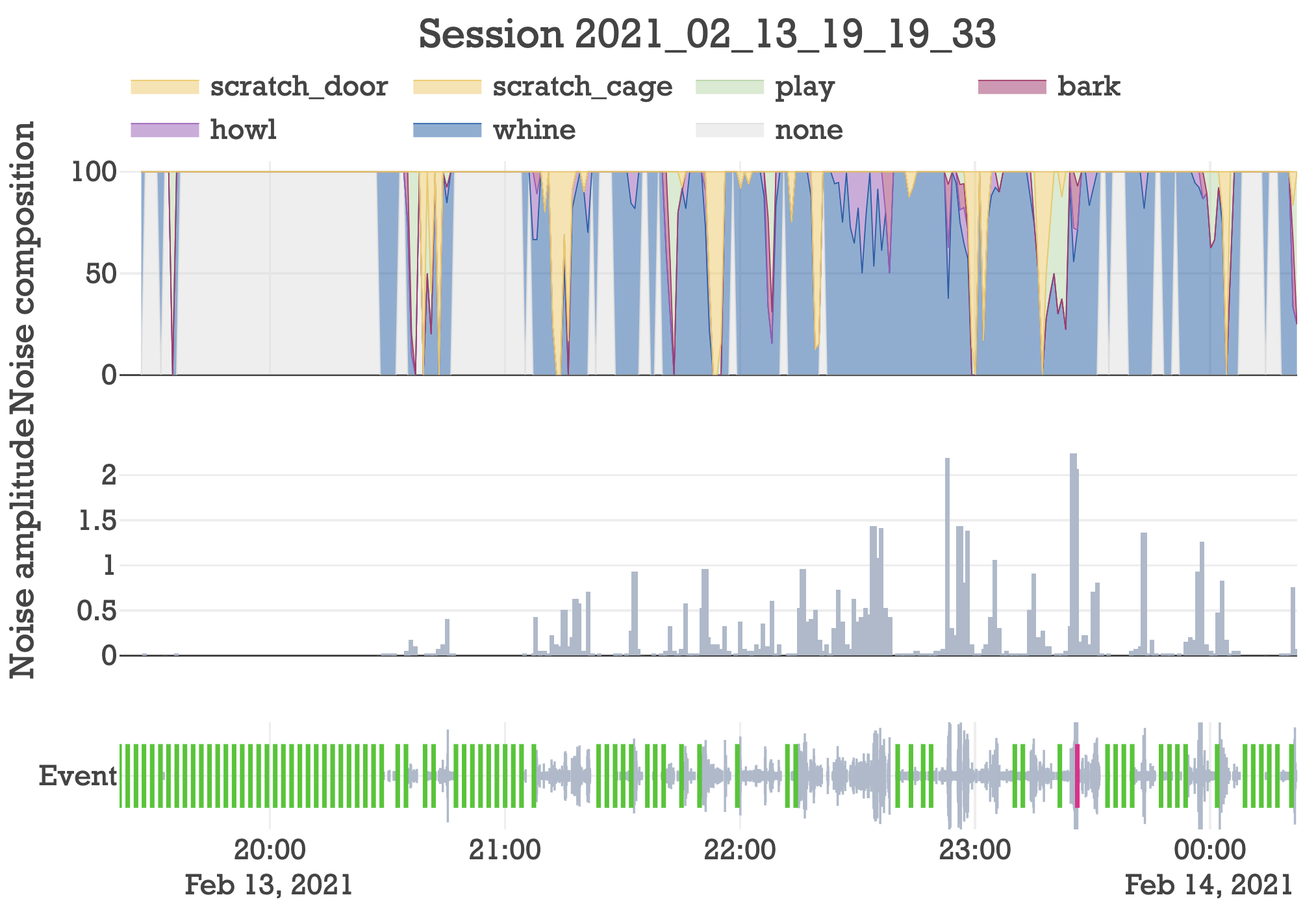
In the first post of this series, I made a virtual dog-sitter that detects audio events, responds to them, and stores them in a database that can be interactively visualized.
Using this dog-sitter (github here), I’ve been tracking the behavior of my girlfriend’s dog (Maple) when we leave her alone in the apartment.
I ended that post saying I would report back after acquiring a lot more data and there are a few logistical updates on that front.
First, it is no longer just Maple we are tracking. We decided that Kourtney’s other dog, Dexter (pictured above), should also be in the room. Originally we separated them based on anecdotal evidence that they barked more when together than when separated. As the data in this post will tell us, keeping them together is a very good idea.
Second, we don’t lock Maple in the crate anymore. This way she can interact and play with Dexter, and pick up new hobbies like destroying our bedroom door (more on that later).
Finally, there were some complications, which means I don’t have as much data as I wanted. Highlights include: I accidentally deleted about a month of data, the volume knob on my microphone changed and went unnoticed for a month, and my calibration system for event detection kept event rates inconsistent across sessions. All of this is sorted out now.
So there isn’t enough data to do a comprehensive analysis on the dogs’ improvement over time, and whether or not praising/scolding has an effect on their behavior. Not yet anyways.
Creating an audio classifier
While I wait another couple months for the data to pour in, I decided that being able to classify audio events could greatly increase the accuracy and capabilities of the dog-sitter.
In the last post I developed flowcharts to determine when the dog-sitter should intervene with pre-recorded audio that either praises or scolds the dog. The logic relied on the assumption that loud is bad and quiet is good. Yet if I could classify each audio event, I could step away from this one dimensional paradigm and begin developing more nuanced responses that understand the sentiment of the audio.
For example, whining could trigger a console response. Playing could trigger an encouragement response. Implementing this with the old paradigm would be impossible, because whining and playing produce similar levels of noise.
So that’s one thing an audio classifier would enable: nuanced response.
Another thing it would enable is protection against non-dog audio. The dog-sitter may detect undesirable noise from nondescript sources, like a nearby lawnmower, a person talking in the alley, a dump truck beeping. If I train a good classifier, I could filter out non-dog audio from ever entering my databases. This would filter bad data out of downstream analyses, and prevent any mishaps like scolding a dog because of a lawnmower.
And finally, creating a classifier would greatly improve the ability to understand what happens when I leave. After returning home, I would be able to immediately assess in a highly-resolved manner how well the dogs behaved while I was gone.
Deciding on a classifier algorithm
Don't make anything more complicated than it needs to be.
In my opinion, this quote should be attributed to the random forest algorithm. There is really no point starting with any other classifying algorithm. If the classifier is bad, I’ll try something more complicated.
Moving on.
Section I: Data transformation
Unfortunately, I can’t just throw the audio data into a random forest and be done with it. The data needs to be wrangled and transformed into a suitable format that’s consistent across samples and pronounces distinguishable features.
Moving forward, I’ll use these two events as examples.
The first is a door scratch:

The second is a whine:
Using the maple API
I found these events using an interactive plot generated with
./main.py analyze --session 2021_02_13_19_19_33
Once I found these two events, I plotted and exported the audio/text files using the SessionAnalysis class in the maple.data module:
from maple.data import SessionAnalysis
session = SessionAnalysis(path='data/sessions/2021_02_13_19_19_33/events.db')

session.plot_audio_event(160)
session.save_event_as_wav(event_id=160, path='door_scratch.wav')
session.save_event_as_txt(event_id=160, path='door_scratch.txt')

session.plot_audio_event(160, xlim=(0, 4.53))
session.save_event_as_wav(event_id=689, path='whine.wav')
session.save_event_as_txt(event_id=689, path='whine.txt')
session.disconnect()
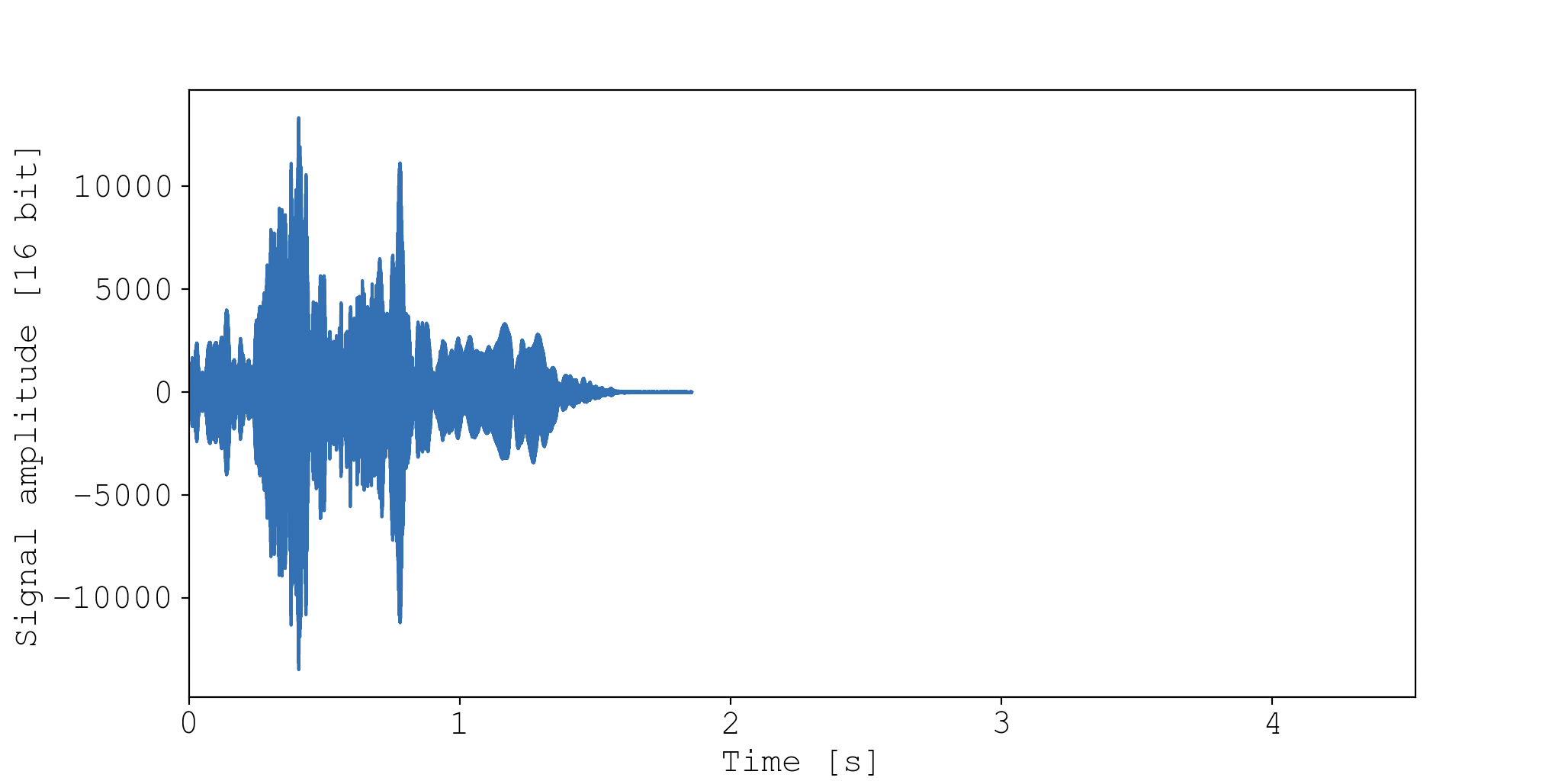
For anyone who doesn’t work with audio files, the data is simple. Audio signal is just a 1D array, where the value of each point is proportional to the pressure/strength of the sound. As you move through the array, you’re moving through time at a specified sampling rate. In my recordings I chose a standard sampling rate of 44100 Hz.
Why 44100 Hz? The human ear can perceive sound waves up to around 20,000 Hz. But resolving a sinusoidal wave requires sampling frequency that is at least double the wave’s frequency. Hence we have 44100 Hz.
Denoising
There are some sources of noise that I have to contend with. Sometimes I leave a (non-rotating) fan on in the room that the mic picks up. Second, there exists some inherent hiss from the microphone. Since both of these noise sources are static (non-dynamic), applying some simple spectral gating can significantly reduce noise. I did exactly this using the python module noisereduce.
Here’s a demonstration of how effective the denoising is. First is raw, second is denoised.
This denoising procedure requires a sample of the background audio, so at the start of a session recording, a 2-second audio clip of the background noise is recorded during calibration. Event audio is then denoised upon detection using this background audio sample. This means the audio used for training and classification has already been denoised.
Data chunking
Each audio event (sample) has a unique length (number of features), yet most classifiers demand that every sample must have the same number of features.
To deal with this, I decided each audio event would be split into equal sized chunks and the classifier would classify chunk-by-chunk.
What length of time should each chunk be? I didn’t want to exclude any events that were shorter than the chunk size, so I took a look at the distribution of event lengths for some random session.
import matplotlib.pyplot as plt
from maple.data import SessionAnalysis
session = SessionAnalysis(path='data/sessions/2021_02_13_19_19_33/events.db')
plt.hist(session.dog['t_len'], bins=300)
plt.yscale('log')
plt.xlabel('event length [s]')
plt.show()
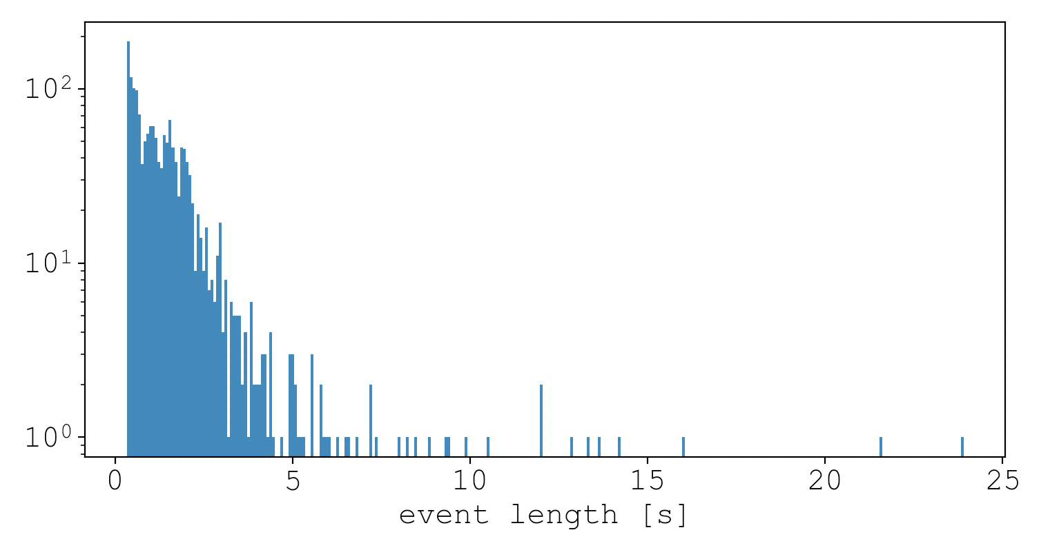
It seems most event times are less than 2.5 seconds, and events are most frequently seen between 0.3s and 0.5s. To make sure events are composed of at least one chunk, I opted to use a chunk size of 0.25s. Alternatively I could have picked a larger chunk size and zero-padded shorter events such that they contained at least one chunk.
The minimum event length time
If you’re wondering why there are no events lower than 0.33s, it has to do with the event detection heuristics. If I used different values, by editing the config file, the minimum event length would have been different. Here are the settings I used for this session (and all sessions):
[detector]
# Standard deviations above background noise to consider start an event
event_start_threshold = 4
# The number of chunks in a row that must exceed event_start_threshold in order to start an event
num_consecutive = 4
# Standard deviations above background noise to end an event
event_end_threshold = 4
# The number of seconds after a chunk dips below event_end_threshold that must pass for the event to
# end. If during this period a chunk exceeds event_start_threshold, the event is sustained
seconds = 0.25
# If an event lasts longer than this many seconds, everything is recalibrated
hang_time = 180
Frequency or time? Answer: both
I want to represent the data so that distinguishable features are accentuated for the classifier. Thinking in these terms, audio has two really important features: time and frequency.
Above is the 1D audio signal for the door scratching event. This plot basically illustrates how energy is spread along the axis of time. And there is clearly distinguishing information in this view. For example, we can see that my door is being destroyed in discrete pulses that are roughly equally spaced through time.
But frequency-space also holds critical information. We can visualize how energy is spread across the axis of frequency by calculating a Fourier transform of both events:
from maple.data import SessionAnalysis
session = SessionAnalysis(path='data/sessions/2021_02_13_19_19_33/events.db')
session.plot_audio_event_freq(160)
session.plot_audio_event_freq(689)
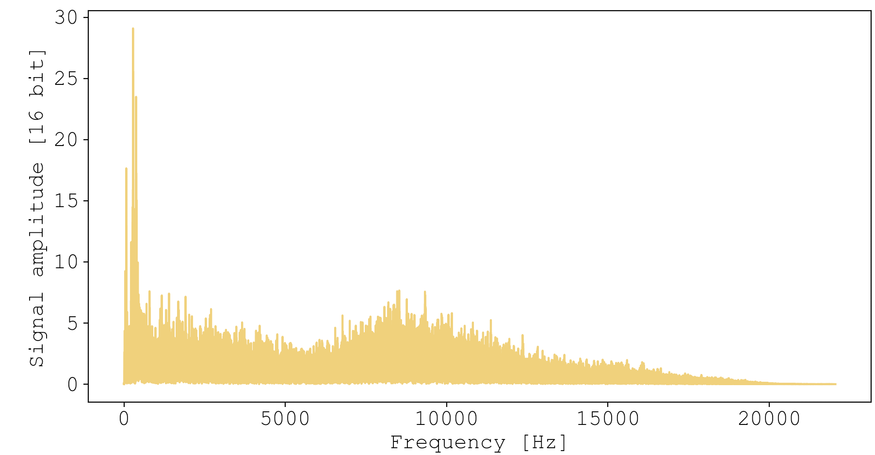
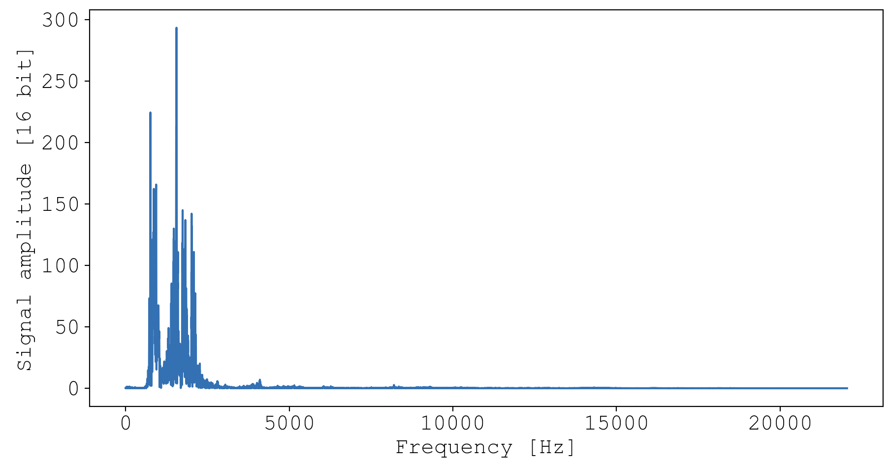
You can really see how my door is being destroyed over a wide range of frequencies. If you listen carefully to the audio, you can hear the bassline and the high hat. In comparison, Maple’s whine is much more concentrated in frequency space, localized to a range of about 500-2500 Hz. This is reflected in the relative pureness of the audio, giving that whistley sort of sound.
Clearly, time and frequency are giving complementary information that the classifier should use both of. To accomplish this, I decided to transform the data into spectrograms, where the $x-$axis is time and the $y-$axis is frequency. This shows how energy is spread across time and frequency space.
from maple.data import SessionAnalysis
session = SessionAnalysis(path='data/sessions/2021_02_13_19_19_33/events.db')
session.plot_audio_event_spectrogram(160, log=True)
session.plot_audio_event_spectrogram(689, log=True)
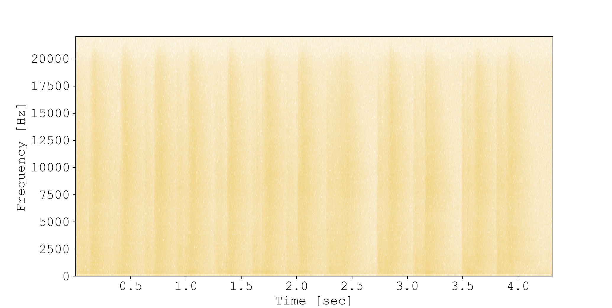
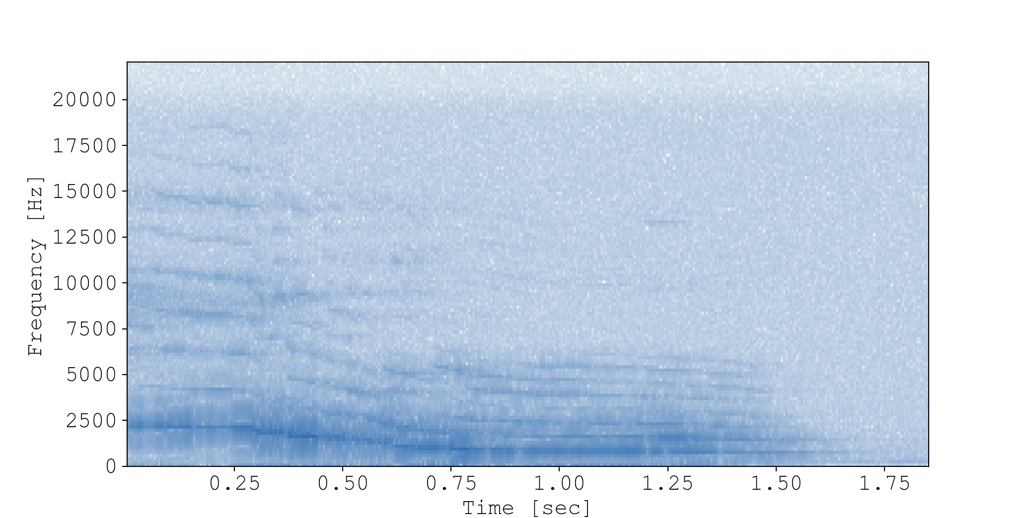
Note that I log-transformed the signal with log=True so that low values are visualizable.
This new view simultaneously illustrates distinguishing features in both time- and frequency-space, and the results are very promising. Look at how different the spectrograms look! And they are very informative. In the whine event, you can really see Maple’s pitch starts high and ends low, which perfectly matches the perceived audio.
Keep in mind that I’ve shown the spectrograms for the entire audio event. But the plan is to slice each audio event into 0.25 second samples, and then calculate spectrograms for each. This ensures each sample has the same number of features (length).
As seen, a spectrogram is a 2D matrix of data, but a classifier expects samples that are 1D. I solve this by flattening each spectrogram by joining all the rows of data into one long 1D array. For example, here is what the first chunk of the whine event ultimately looks like to the classifier:
import matplotlib.pyplot as plt
from maple.data import SessionAnalysis
from maple.audio import get_spectrogram

session = SessionAnalysis(path='data/sessions/2021_02_13_19_19_33/events.db')
subevent_audio = session.get_subevent_audio(event_id=689, subevent_id=0, subevent_time=0.25)
_, _, S = get_spectrogram(subevent_audio, log=False, flatten=True)

plt.plot(S, c='#165BAA')
plt.ylabel('Signal amplitude [16 bit]')
plt.xlabel('Flattened axis')
plt.show()
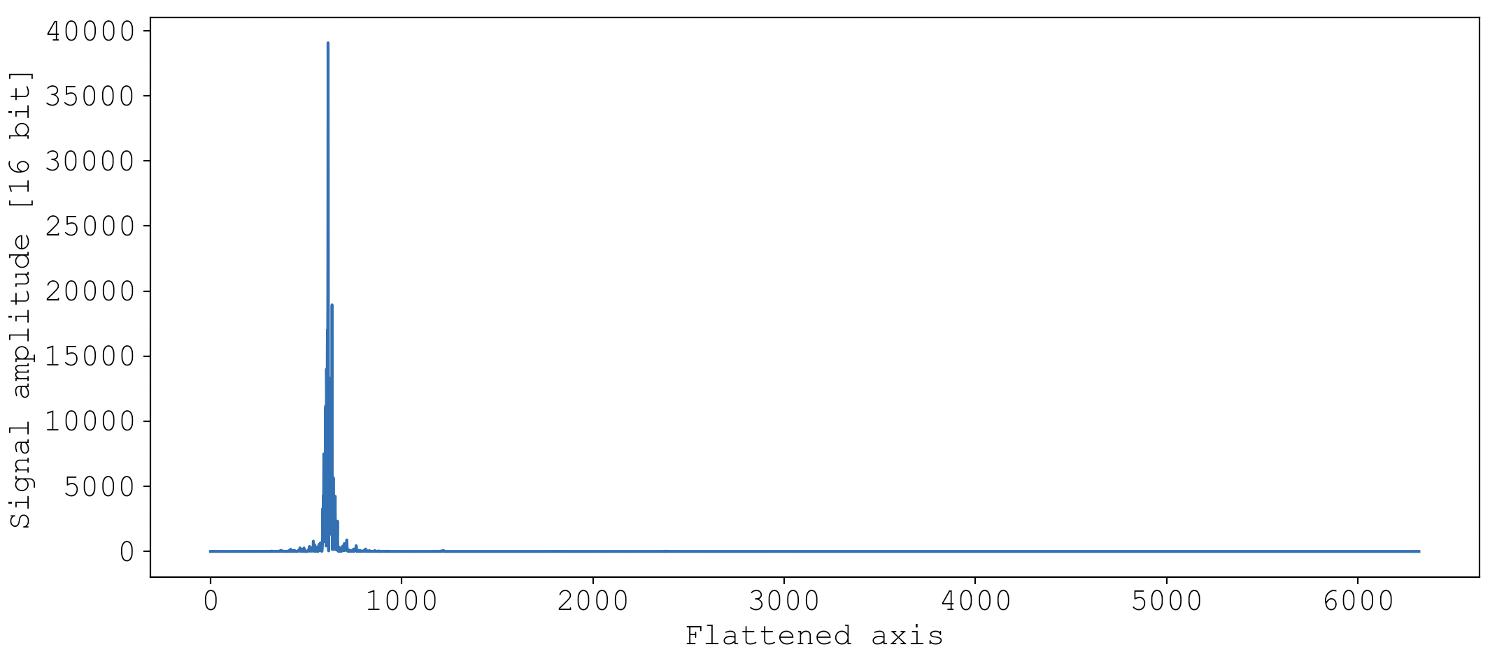
This may not look as informative as the 2D heatmaps shown above, but it contains exactly the same information.
Transformation summary
A brief summary is in order.
- Audio clips are denoised with spectral gating to remove static noise
- Audio clips are segmented into 0.25 second chunks and will be classified chunk-by-chunk
- Each chunk is transformed into a spectrogram to accentuate the most important qualities of sound: amplitude with respect to time, and amplitude with respect to pitch.
- The spectrograms are flattened into 1D arrays for the sake of the classifier
Section II: Labeling
The random forest algorithm requires training data. I considered two options for obtaining training data:
- Use a database of labelled dog audio, assuming such a dataset exists freely on the internet somewhere.
- Manually label a subset of the audio events I have recorded over the last several months.
Ultimately, I decided on option 2, but option 1 is not without merits.
First of all, option 1 doesn’t require manual labeling, which is a huge investment of time. Second, such a broad database would presumably have data recorded under a multitude of audio settings and for a multitude of dogs, which is good and bad. It’s good because it makes the classifier more suitable for productionalization for when different mic settings, room acoustics, and dogs would in theory be used. But it also is bad because accuracy will suffer in comparison to a dataset trained specifically on Maple and Dexter with consistent mic settings and acoustic environments.
Ultimately this is what swayed me to option 2. Additionally, manually labelled data reduces constraints because I can create whichever labels I want. For example, a pre-labeled database would be unlikely to have a scratch_door label, and if it did, it would be unlikely to sound like my particular door.
Picking labels
Before going through the process of manually labelling data, I needed to decide on the set of labels to use. After reviewing the audio, Kourtney and I decided on these 6 labels.
Whine
At this point, you’re familiar with the whine. This is primarily a Maple special, although Dexter is also well-versed in the art.
Howl
The howl is a distinct escalation of the whine, exhibited exclusively by Maple.
Bark
The bark space is dominated by Dexter. It’s characterized by its high pitch, and being miserable to listen to.
You should turn your volume down.
Play
Maple and Dexter often play together. It may surprise you that it sounds like this:
Usually playing means tug of war with a toy, biting each other’s ears, or chasing each other.
Door scratch
This one you’ve already heard. I haven’t collected any direct evidence for who is responsible for ruining my door, but I suspect it is Maple.
None
This class is a catch-all for events that are not made by the dogs, or don’t fit into the other classes. For example, here is me greeting Dexter after returning home:
The more audio events I can label with this class, the more protection I will have against false-positives.
With a set of labels, it’s time to label a boat-load of data.
Labeling
Manual labelling is so laborious that I wanted to streamline the process as best I could. Basically, I needed something that would subsample events from a collection of session databases, play them to me, splice them into chunks, and then store the label I attribute into a table. This is all handled by the class LabelAudio in the maple.classifier module.
I extended the command line utility to use the class with the following command:
./main.py label --label-data label_data.txt --session-paths training_session_paths
Here’s a demo.
With the labeler in hand, my initial goal was to label 10,000 audio chunks. But of the 50,621 audio chunks at my disposable, Kourtney and I were able to withstand labelling just 2,745 audio chunks before giving up. Hopefully it’s enough.
Section III: Training
The next step was to actually create and validate a random forest with this labelled data.
Class description
Basically, I needed to load in the label data, transform the audio into spectrograms, split the data into training and validation sets, build the classifier using the training set, validate the classifier with the validation set, and save the model for further use. To do this, I wrote a class called Train which lives in the maple.classifier module. You can peruse it here at your leisure if you want the full story. Here I’ll summarize some things.
This class starts in the __init__ method by loading in the label data as a dataframe.
...
self.label_data_path = Path(args.label_data)
self.label_data = pd.read_csv(self.label_data_path, sep='\t')
...
The label data looks like this:
| session_id | event_id | subevent_id | t_start | t_end | label | date_labeled |
|---|---|---|---|---|---|---|
| 2021_03_05_20_10_07 | 430 | 0 | 0.0 | 0.25 | bark | 2021-03-15 22:41:29.135011 |
| 2021_03_05_20_10_07 | 430 | 1 | 0.25 | 0.5 | none | 2021-03-15 22:41:44.855221 |
| 2021_01_19_13_59_02 | 39 | 0 | 0.0 | 0.25 | howl | 2021-03-15 22:42:07.451854 |
| 2021_01_19_13_59_02 | 39 | 1 | 0.25 | 0.5 | howl | 2021-03-15 22:42:08.434805 |
| 2021_01_19_13_59_02 | 39 | 2 | 0.5 | 0.75 | howl | 2021-03-15 22:42:09.842651 |
| 2021_01_19_13_59_02 | 39 | 3 | 0.75 | 1.0 | howl | 2021-03-15 22:42:10.959118 |
| 2021_01_19_13_59_02 | 39 | 4 | 1.0 | 1.25 | howl | 2021-03-15 22:42:12.299899 |
| 2021_01_19_13_59_02 | 39 | 5 | 1.25 | 1.5 | howl | 2021-03-15 22:42:13.635911 |
| 2021_01_19_13_59_02 | 39 | 6 | 1.5 | 1.75 | howl | 2021-03-15 22:42:44.608062 |
| 2021_02_11_16_56_39 | 7 | 0 | 0.0 | 0.25 | whine | 2021-03-15 22:42:55.567570 |
| … | … | … | … | … | … | … |
Notice that the actual audio data isn’t in here, it’s merely referenced by session_id, event_id, and subevent_id. In theory, I could have added the audio as another column like this:
| audio |
|---|
| 216,224,222,224,223,209,187,135,82,4… |
| -10,-3,13,33,37,16,8,22,31,52,73,8… |
| 76,136,175,185,156,105,44,-40,-112,-… |
| 192,196,200,209,213,228,242,244,251,… |
| 39,41,39,59,59,55,52,67,103,130,137… |
| 30,49,51,40,18,-27,-2,24,-39,-119,-… |
| -222,62,144,-71,-212,-45,152,65,-135,… |
| 9,45,88,155,88,-47,-78,-37,0,-52,-1… |
| 6,9,4,-20,-31,-34,-30,-27,-25,-18,-… |
However this is pretty messy and a waste of space. Why duplicate the audio when it’s already stored in the session databases? Furthermore, I’ve written an API that makes accessing the data easy, so why not use it?. To associate these labels to their underlying audio data, I created a dictionary of SessionAnalysis instances, one for each session:
...
self.dbs = {}
session_ids = self.label_data['session_id'].unique()
for session_id in session_ids:
    self.dbs[session_id] = data.SessionAnalysis(name=session_id)
...
Then, I wrote methods to query the underlying audio data of any audio chunk, which I call a subevent:
def get_event_audio(self, session_id, event_id):
    return self.dbs[session_id].get_event_audio(event_id)


def get_subevent_audio(self, session_id, event_id, subevent_id):
    event_audio = self.get_event_audio(session_id, event_id)

    subevent_len = int(self.subevent_time * maple.RATE)
    subevent_audio = event_audio[subevent_id * subevent_len: (subevent_id + 1) * subevent_len]

    return subevent_audio
Now I can easily access the audio for any subevent. For example, the first label data is
| session_id | event_id | subevent_id | t_start | t_end | label | date_labeled |
|---|---|---|---|---|---|---|
| 2021_03_05_20_10_07 | 430 | 0 | 0.0 | 0.25 | bark | 2021-03-15 22:41:29.135011 |
The audio can be accessed with
self.get_subevent_audio('2021_03_05_20_10_07', 430, 0)
By the way, if you go down the rabbit hole, this audio data is ultimately obtained by an SQL query using the sqlite3 python API.
Preparing the data is done with self.prep_data.
def prep_data(self, transformation='spectrogram'):
    """Establishes the training and validation datasets

    This method sets the attributes `self.X`, and `self.y`

    Parameters
    ==========
    transformation : str, 'spectrogram'
        Pick any of {'spectrogram', 'none', 'fourier'}.
    """

    a = self.label_data.shape[0]

    if transformation == 'spectrogram':
        transformation_fn = self.get_subevent_spectrogram
        b = self.get_spectrogram_length()
    elif transformation == 'none':
        transformation_fn = self.get_subevent_audio
        b = self.get_audio_length()
    elif transformation == 'fourier':
        transformation_fn = self.get_subevent_fourier
        b = self.get_fourier_length()
    else:
        raise Exception(f"transformation '{transformation}' not implemented.")

    self.X = np.zeros((a, b))
    self.y = np.zeros(a).astype(int)

    for i, subevent in self.label_data.iterrows():
        label = self.label_dict[subevent['label']]
        self.y[i] = label

        self.X[i, :] = transformation_fn(
            session_id = subevent['session_id'],
            event_id = subevent['event_id'],
            subevent_id = subevent['subevent_id'],
        )

    if self.log:
        self.X = np.log2(self.X)
This method sets the attributes self.X and self.y. Each row of self.X is the data for each audio chunk, and each element of self.y is a numerical label corresponding to each of the 6 classes. transformation will define the contents of each row. If transformation='spectrogram', each row is the flattened spectrogram of an audio chunk. If transformation='fourier', each row is the Fourier amplitude spectrum of an audio chunk. And finally, if transformation='none', each row is the raw audio signal. I find the ability to train using any of these transformations very exciting because I can directly compare performance depending on which transformation is used.
With self.X and self.y defined, the model can be trained. This is done with self.fit_data which is a sklearn.ensemble.RandomForestClassifier wrapper.
def fit_data(self, *args, **kwargs):
    """Trains a random forest classifier and calculates an OOB model score.

    This method trains a model that is stored as `self.model`. `self.model` is a
    `sklearn.ensemble.RandomForestClassifier` object. The model score (fraction of correctly
    predicted validation samples) is stored as `self.model.xval_score_`

    Parameters
    ==========
    *args, **kwargs
        Uses any and all parameters accepted by `sklearn.ensemble.RandomForestClassifier`
        https://scikit-learn.org/stable/modules/generated/sklearn.ensemble.RandomForestClassifier.html
    """

    self.model = RandomForestClassifier(*args, **kwargs)
    self.model.fit(self.X, self.y)
The model is trained and stored as self.model and a quality score using out-of-bag samples (a unique quality of the random forest classifier) is stored as self.model.oob_score_.
Once the model has been created, it can be saved for later use with self.save_model, which makes use of joblib.
    def save_model(self, filepath):
        """Saves `self.model` as a file with using `joblib.dump`

        Saves `self.model`, which is a `sklearn.ensemble.RandomForestClassifier` object, to
        `filepath`.  Before saving, some the `sample_rate`, `subevent_time`, `subevent_len`, and
        whether the spectrogram was log-transformed (`log`) are stored as additional attributes of
        `self.model`.

        Parameters
        ==========
        filepath : str, Path-like
            Stores the model with `joblib.dump`
        """

        self.model.log = self.log
        self.model.subevent_time = self.subevent_time
        self.model.sample_rate = maple.RATE
        self.model.subevent_len = int(self.model.subevent_time * self.model.sample_rate)
        joblib.dump(self.model, filepath)
This provides convenient access to the model so that at any time, the model can be loaded with
import joblib
model = joblib.load(path)
As a matter of convenience, I also store training and data parameters as attributes of self.model. For example, the sampling rate of the audio, the size of each data chunk, and the transformation type are all stored directly in self.model which makes this information available when the model is loaded at a later date.
The totality of the model-building procedure is glued together with self.run.
def run(self):
    """Run the training procedure

    This method glues the procedure together.
    """

    self.prep_data(spectrogram=True)

    self.fit_data(
        oob_score = True,
    )

    self.save_model(self.model_dir / 'model.dat')
    self.disconnect_dbs()
Performance
This is the fun part. How good is the model? I wanted to address this question from several standpoints.
- Hyperparameter tuning: What are the optimal parameters for the model fit?
- Data transformation comparisons: Does the spectrogram data outperform the raw audio signal? How about the Fourier signal?
- Quantity of training data: Would labeling more data significantly increase accuracy or have I reached the point of diminishing returns?
But first, let’s just get a rough idea of how good the model is using out-of-the-box parameters, aka sklearn’s defaults. I extended the command line to include a train mode, so I can train the data like so.
./main.py train --label-data label_data.txt --model-dir model
This created a model file under model/model.dat. Loading up the model and printing out the out-of-bag validation score yields
import joblib
model = joblib.load('model/model.dat')
print(model.oob_score_)
>>> 0.8506375227686703
It correctly labelled 85% of the validation dataset. In my opinion, that’s really good given such a small training dataset.
Hyperparameter tuning
The default model parameters did a pretty good job, but let’s see if tuning the hyperparameters can improve performance.
The plan is to do a hyperparameter grid search to see what kind of model performance improvements can be achieved. However, before doing that there is one parameter of especial interest, since it greatly affects the speed of training: the number of trees.
Random forest classifiers create a forest of decision trees, and for achieving the highest accuracy, more trees is better. Let’s call the number of trees $n$. Increasing $n$ will statistically speaking increase model accuracy, however there is a law of diminishing returns and this comes at the cost of fit speed.
Choosing $n=10,000$ would be a bad idea for the hyperparameter grid search, since it would take minutes to generate each model. So to increase my search space, I wanted to pick the lowest number of trees possible so that model generation is fast, yet the results are good enough to make reliable decisions from. Then, the plan is to hold the number of trees constant for the grid search and vary all of the other hyperparameters.
So how many trees should I pick? I wrote a quick script that prepares the data using the Train class and then generates models for varying $n$. For each $n$ value I used a 3-fold cross validation to reduce the effect of overfitting to any particular data subset. Then, I plotted the mean and standard error of the cross-validation scores at each $n$ along with the mean time that it took to fit each model.
#! /usr/bin/env python
import argparse
import numpy as np
import matplotlib.pyplot as plt

from maple.classifier import Train
from sklearn.ensemble import RandomForestClassifier
from sklearn.model_selection import GridSearchCV

args = argparse.Namespace(label_data = 'label_data.txt', model_dir = 'none')
train = Train(args)
train.prep_data()

param_grid = {
    'n_estimators': np.logspace(start=0, stop=3, num=30, dtype=int),
}

model_search = GridSearchCV(
    estimator = RandomForestClassifier(),
    param_grid = param_grid,
    cv = 3,
    verbose = 2,
    n_jobs = -1,
)
model_search.fit(train.X, train.y)

# Plotting

model_df = pd.DataFrame(model_search.cv_results_)
n_trees = model_df['param_n_estimators'].values
mean_scores = model_df['mean_test_score'].values
std_err_scores = model_df['std_test_score'].values/np.sqrt(len(n_trees))
fit_times = model_df['mean_fit_time'].values
std_err_times = model_df['std_fit_time'].values/np.sqrt(len(n_trees))

fig, ax1 = plt.subplots()

color = 'tab:red'
ax1.set_title('Tradeoff of fit time vs accuracy')
ax1.set_xlabel('Number of trees')
ax1.set_ylabel('Cross-validation score', color=color)
ax1.set_xscale('log')
ax1.errorbar(n_trees, mean_scores, yerr=std_err_scores, capsize=4.0, fmt='--', color=color)
ax1.tick_params(axis='y', labelcolor=color)

ax2 = ax1.twinx()

color = 'tab:blue'
ax2.set_ylabel('Fit time [s]', color=color)
ax2.errorbar(n_trees, fit_times, yerr=std_err_times, capsize=4.0, fmt='--', color=color)
ax2.tick_params(axis='y', labelcolor=color)

fig.tight_layout()
plt.show()
Running the script produces a plot that illustrates the increase in accuracy (shown in red) as a function of $n$, the number of trees, at the expense of fit time (shown in blue).
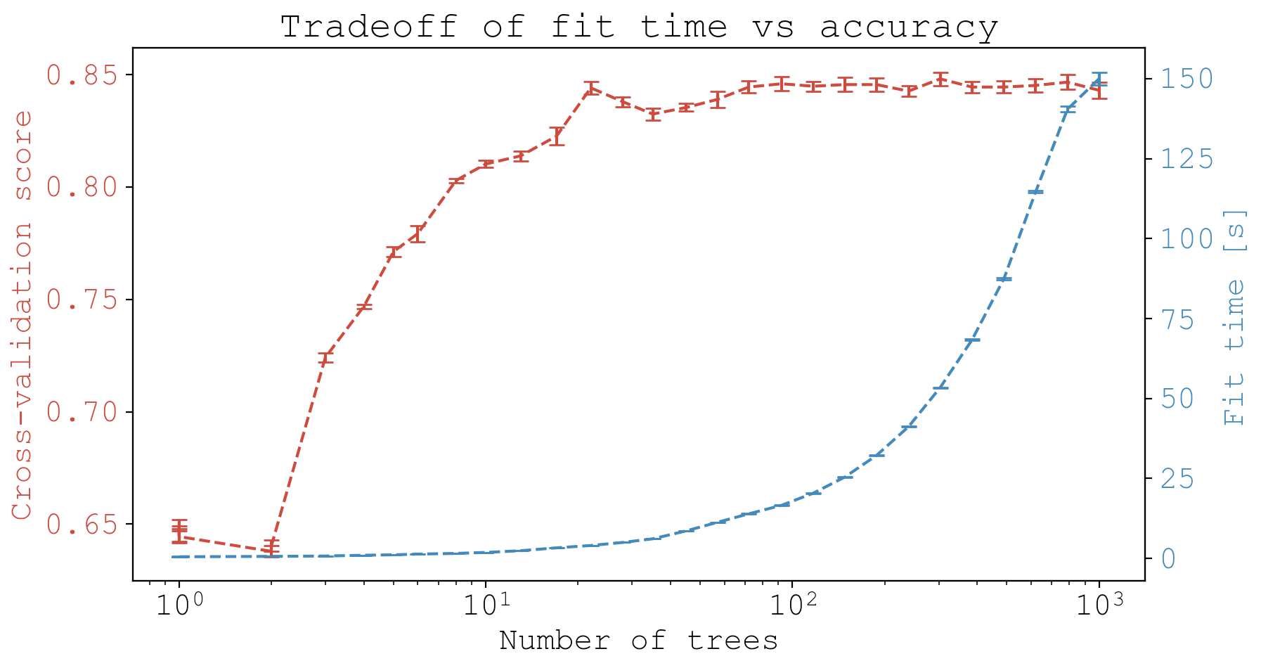
So as expected, the more trees the better, but there is definitely a point of diminishing returns past around 20 trees. And this comes at substantial time cost, where in blue we can see the model fit time increases exponentially as a function of $n$.
Overall, these data are showing me it wouldn’t be a bad idea to use $n=30$ for the hyperparameter grid search.
To do the grid search, I took a look at the sklearn.RandomForestClassifier docs as well as this blog and ultimately decided on the following parameter grid:
param_grid = {
    'n_estimators': [30],
    'max_features': ['sqrt', 'log2'],
    'max_depth': list(np.arange(5, 100, 5).astype(int)) + [None],
    'min_samples_split': [2, 5, 10, 20],
    'min_samples_leaf': [1, 2, 4, 8],
}
That’s 640 different parameter combinations, and with a 5-fold cross-validation per parameter set, I needed to generate 3200 different models. That’s why picking the smallest $n$ possible is so important. I ran the grid search with the following script, which took about an hour to run (I estimate it would have taken 3 hours for $n=200$ and 9 hours for $n=500$).
#! /usr/bin/env python
import argparse
import numpy as np

from maple.classifier import Train
from sklearn.ensemble import RandomForestClassifier
from sklearn.model_selection import GridSearchCV

args = argparse.Namespace(label_data = 'label_data.txt')
train = Train(args)
train.prep_data()

param_grid = {
    'n_estimators': [30],
    'max_features': ['sqrt', 'log2'],
    'max_depth': list(np.arange(5, 100, 5).astype(int)) + [None],
    'min_samples_split': [2, 5, 10, 20],
    'min_samples_leaf': [1, 2, 4, 8],
}

model_search = GridSearchCV(
    estimator = RandomForestClassifier(),
    param_grid = param_grid,
    cv = 5,
    verbose = 2,
    n_jobs = -1,
)
model_search.fit(train.X, train.y)

df = pd.DataFrame(model_search.cv_results_).sort_values(by='rank_test_score')
cols = ['mean_fit_time', 'mean_score_time', 'mean_test_score'] + [x for x in df.columns if x.startswith('param') and not x.endswith('param')]
df = df[cols]
df.to_csv('hyperparameter_tuning_results.txt', sep='\t', index=False)
The output of this script is a dataframe. First, I looked at the model performances by ordering them according to their rank, and noticed there appears to be 3 apparent regimes of model quality, that I’ve colored below.
In [1]: plt.plot(df['rank_test_score'], df['mean_test_score']); plt.xlabel('Rank'); plt.ylabel('Accuracy'); plt.show()
![]()
I wondered if there were any keystone parameters that partition the models into these three regimes. So I looked at the most common parameter value chosen for each of the three regimes.
In [2]: df.loc[df['rank_test_score'] < 20, 'regime'] = 'top'
In [3]: df.loc[(df['rank_test_score'] >= 20) & (df['rank_test_score'] < 600), 'regime'] = 'middle'
In [4]: df.loc[df['rank_test_score'] >= 600, 'regime'] = 'bottom'
In [5]: counts = df.groupby('regime')[['param_max_features', 'param_max_depth', 'param_min_samples_leaf', 'param_min_samples_split']].describe()
In [6]: counts = counts.iloc[:, counts.columns.get_level_values(1).isin(['count', 'freq', 'top'])]
In [7]: most_common = counts.iloc[:, counts.columns.get_level_values(1) == 'top'].droplevel(1, axis=1).transpose()
In [8]: most_common
Out[8]:
                        bottom middle   top
param_max_features        log2   log2  sqrt
param_max_depth              5     30    40
param_min_samples_leaf       8      4     2
param_min_samples_split     20     20     5
Surprisingly, this partitioning according to rank is 100% interpretable.
Take a look at max_features.
In [9]: most_common.loc['param_max_features']
Out[9]:
bottom    log2
middle    log2
top       sqrt
Name: param_max_features, dtype: object
The most commonly seen max_features in the top regime is sqrt, whereas the most common in the middle and bottom regimes both have max_features equal to log2. In fact, the best ranking model with max_features equal to log2 ranks 101st. This indicates that sqrt is strongly favored for the spectrogram transformation, and that max_features is a very important distinguishing hyperparameter.
Moving on to the other 3 parameters, here I’ve plotted the most common value seen for each regime.
In [10]: most_common.iloc[1:].plot.bar(rot=10); plt.tight_layout(); plt.ylabel('value'); plt.show()
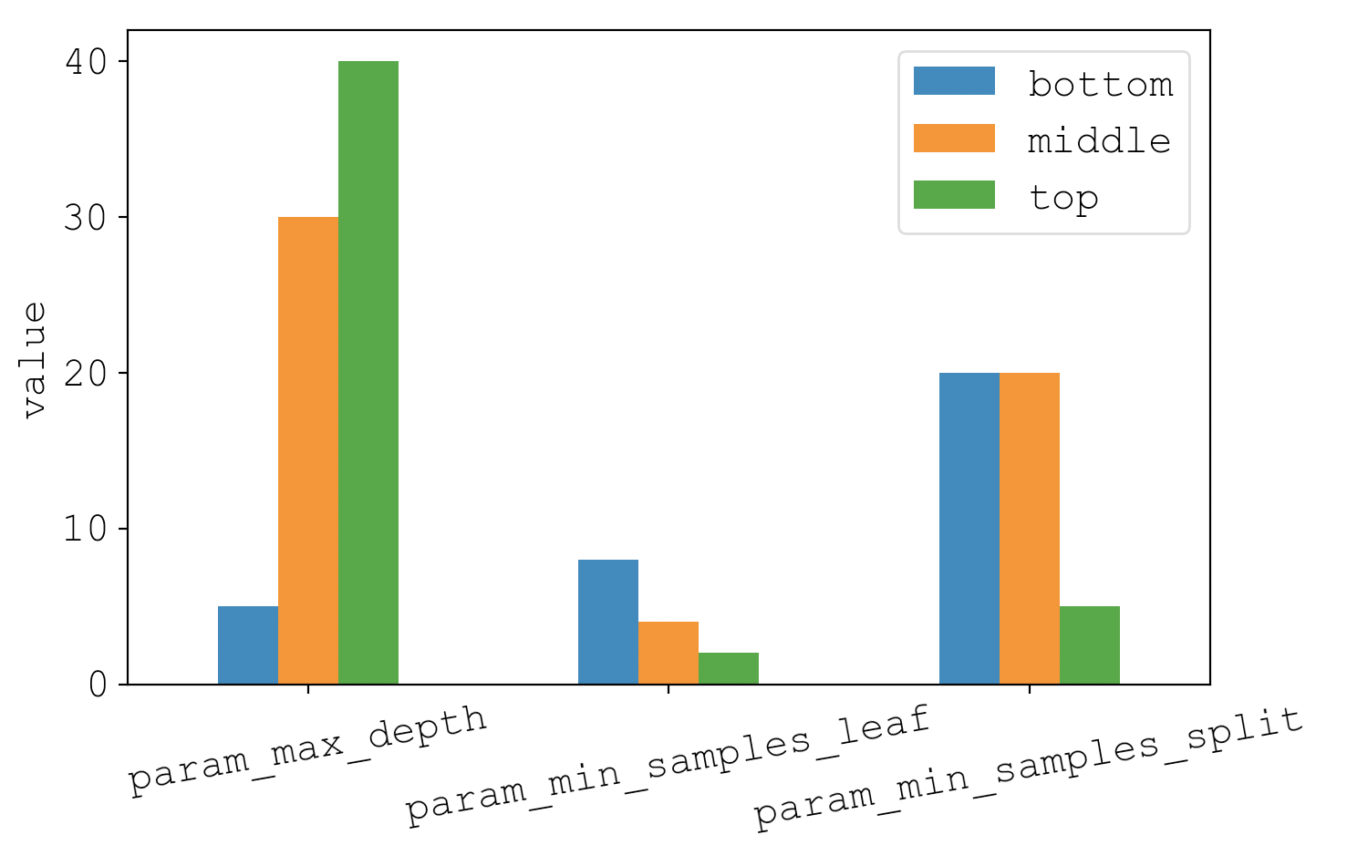
On the far left is max_depth, where we see a clear increase in max_depth as the models get better and better. In fact, around 75% of models in the bottom regime have a max_depth of 5. Similarly for min_samples_leaf and min_samples_split, we see that the middle and bottom regimes consistently have high values, and the top regime has low values.
The consistent theme in the trends of max_depth, min_samples_leaf, and min_samples_split is that top-performing models do not want to be constrained in the number of leaves in the decision tree. This makes intuitive sense, but it’s nice to see it in the data.
Based on these findings, I’ve decided to update Train.fit_data to perform a small parameter scan with 10-fold cross validation. The new method looks like this:
def fit_data(self):
    """Trains a random forest classifier and calculates a model score.

    This method trains a bunch of models over a small subset of hyperparameter space based on an
    ad-hoc analysis described here:
    ekiefl.github.io/2021/03/14/maple-classifier/#-hyperparameter-tuning

    For each model setting, a 5-fold cross validation is used. When the most accurate model is
    determined, it is stored as `self.model` and the 5-fold cross validation accuracy is stored
    as self.model.xval_score_.
    """

    model_search = GridSearchCV(
        estimator = RandomForestClassifier(),
        param_grid = {
            'n_estimators': [200],
            'max_features': ['sqrt', 'log2'],
            'criterion': ['gini', 'entropy'],
        },
        cv = 10,
        verbose = 2,
        n_jobs = -1,
    )
    model_search.fit(self.X, self.y)

    self.model = model_search.best_estimator_
    self.model.xval_score_ = model_search.best_score_
Data transformation comparisons
In the data transformation section, I kept harping about how spectrograms would outperform time series audio (time-space) and Fourier spectra (frequency-space) because they resolve both time and frequency components simultaneously. Let’s see if that’s actually true.
Thanks to how general Train.prep_data is, this is really easy to test. To do so, I wrote this little script that calculates models with varying transformations.
#! /usr/bin/env python
import argparse
import pandas as pd

from pathlib import Path
from maple.classifier import Train

trans_settings = [
    ('spectrogram', False),
    ('spectrogram', True),
    ('fourier', False),
    ('fourier', True),
    ('none', False),
]

args = argparse.Namespace(label_data = 'label_data.txt')
train = Train(args)

scores = []
for trans, log in trans_settings:
    train.trans, train.log = trans, log
    train.model_dir = Path(f'model_{trans}' + ('_log' if log else ''))
    train.run(disconnect_dbs = False)
    scores.append(train.model.xval_score_)
train.disconnect_dbs()

results = pd.DataFrame({
    'transformation': list(zip(*trans_settings))[0],
    'log': list(zip(*trans_settings))[1],
    'score': scores
})
print(results.to_markdown())
I was also curious whether or not log-transforming the data could increase accuracy, so that’s in the script too.
The output is a table summarizing the prediction quality for various types of transformations on the audio data:
| transformation | log | score | |
|---|---|---|---|
| 0 | spectrogram | False | 0.852823 |
| 1 | spectrogram | True | 0.850638 |
| 2 | fourier | False | 0.825865 |
| 3 | fourier | True | 0.826958 |
| 4 | none | False | 0.632423 |
It’s great to verify what I’ve been advertising: the spectrogram outperforms the time- and frequency-space transformations. It’s interesting to see how poor the classifier performs when trained on the time series audio signal. As a final observation, log-transforming the data seems to have little effect on performance.
Quantity of training data
So hyperparameter tuning and investigating alternative data transformations did not yield significant increases in classification performance. The only remaining thing to investigate is: should I label more data?
A bigger training dataset is definitely better, but there comes a point where the reward does not match the effort. So before committing to labeling more data, which sucks, I wanted to know how much room there is for improvement. Basically, if $N$ is the size of my training dataset, and $S$ is the model score, I wanted to know where I lie on this learning curve:

To get an idea of where I am on the learning curve, I trained a series of models with a subset of my 2,745 label data and visualized the results. At each fraction of the full data, I’m doing a 5-fold cross validation for 5 trials, where the training data is resampled for each trial.
#! /usr/bin/env python
import argparse
import pandas as pd
import matplotlib.pyplot as plt

from maple.classifier import Train

args = argparse.Namespace(label_data = 'label_data.txt')
train = Train(args)
full_data = train.label_data.copy()

param_grid = {
    'n_estimators': [30],
},

fracs = np.linspace(0.1, 1, 50)
scores = np.zeros(len(fracs))

trials = 5

for i, frac in enumerate(fracs):
    s = np.zeros(trials)
    for t in range(trials):
        train.label_data = full_data.sample(frac=frac).reset_index(drop=True)
        train.prep_data(transformation='spectrogram')
        train.fit_data(param_grid=param_grid, cv=5)
        s[t] = train.model.xval_score_
    scores[i] = np.mean(s)

color = '#9E70B8'
plt.title('Should I keep labeling?')
plt.xlabel('Size of training dataset (N)')
plt.ylabel('Model score (S)', color=color)
plt.plot((full_data.shape[0]*fracs).astype(int), scores, c=color)
plt.yticks(np.round(np.arange(min(scores), max(scores)+0.01, 0.01), 2))
plt.show()
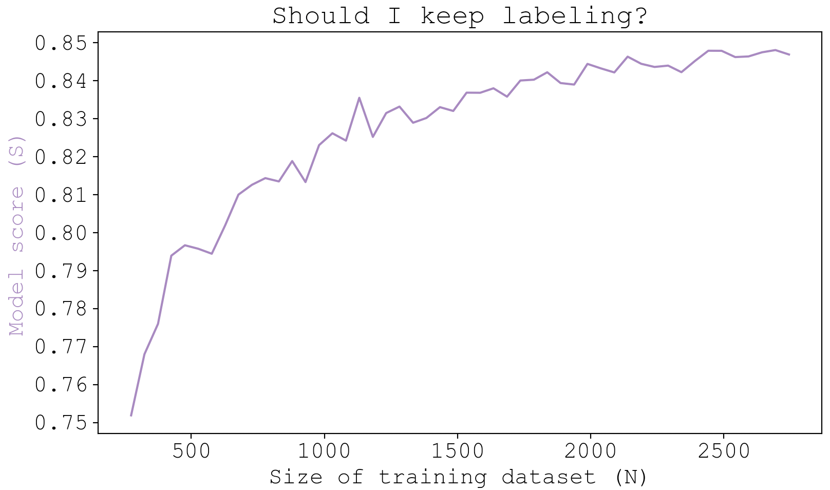
To my eye, it seems like there isn’t much to gain from labeling more data, but I really wanted to see if I could break 86% accuracy, so I decided that I would label up to $N=5000$.
To start labeling more data, I ran the command
./main.py label --label-data label_data.txt --session-paths training_session_paths
75 minutes later, there are now 5,031 labelled audio chunks. Repeating the analysis I ended up with this new learning curve:

The results did not change significantly. Certainly not enough to have justified 75 minutes. It seems like the increase in accuracy was about 0.5-1.0%, bringing the total accuracy just above 85%.
These plots were generated using 30 trees to cut down on run-time, so the final model with 200 trees will produce a slightly higher score.
Final model accuracy
After considering hyperparameter space, alternative data transformations, and doubling the amount of training data, I’ve exhausted all my options. It is time to run one last model: the one I’ll use moving forward:
./main.py train --label-data label_data.txt --model-dir model
This model is produced from a cross-validation grid search of potential models, which has no constraints on tree depth or leaf number, considers 2 alternatives for the max number of features each tree is built from (sqrt and log2), 2 alternatives for splitting criterion (gini and entropy), and a fixed tree number of 200. Each model’s score is determined from a 20-fold cross-validation scheme and the top-ranking model becomes the chosen model.
Loading up the resultant model and printing its score yields a final accuracy of 86.1%
import joblib
model = joblib.load('model/model.dat')
print(model.xval_score_)
>>> 0.8610715866691964
Section IV: Classifying
Training the model is one thing. Using it is another. In this section I will use the model to classify and visualize past audio events from the last several months.
The workhorse for all classification in maple is this simple class (source code):
class Classifier(object):
    def __init__(self, path):
        path = Path(path)
        if not path.exists():
            raise Exception(f'{path} does not exist')

        self.model = joblib.load(path)

        if self.model.scale:
            self.scaler = joblib.load(path.parent / 'scaler.dat')


    def predict(self, event_audio, as_label=False):
        """Given an arbitrary audio length, predict the class"""

        num_chunks = int(len(event_audio) / self.model.subevent_len)
        if not num_chunks:
            return 'none' if as_label else 0

        data = np.zeros((num_chunks, self.model.n_features_))
        for i in range(num_chunks):
            audio_chunk = event_audio[i * self.model.subevent_len: (i + 1) * self.model.subevent_len]
            data[i, :] = self.transform(audio_chunk)

        chunk_predictions = self.model.predict(data)

        # most common
        prediction = np.bincount(chunk_predictions).argmax()
        return labels[prediction] if as_label else prediction


    def transform(self, audio_chunk):
        if self.model.trans == 'spectrogram':
            data = audio.get_spectrogram(audio_chunk, fs=self.model.sample_rate, flatten=True)[2]
        elif self.model.trans == 'fourier':
            data = audio.get_fourier(audio_chunk, fs=self.model.sample_rate)[0]
        elif self.model.trans == 'none':
            data = np.copy(audio_chunk)
        else:
            raise Exception(f"Transformation '{selfmodel.trans}' not implemented for Classifier")

        if self.model.log:
            data = np.log2(data)

        if self.model.scale:
            data = self.scaler.transform(data.reshape(1, -1)).flatten()

        if self.model.norm:
            data = (data - data.mean()) / data.std()

        if np.isnan(data).all():
            # In diabolical cases an audio chunk may have all zeros, which result in nan's that break
            # the predict method.
            data = np.zeros(len(data))

        return data
Classifier is initialized by providing the path to a model. Because Train stored all of the transformation metadata as attributes of the model object (such as whether it was trained on spectrograms, Fourier spectra, or raw audio trans; whether it was log-transformed log; whether it was feature scaled scale; whether the samples were normalized norm), upon loading the model, Classifier knows exactly how it must transform incoming target data.
This means predicting the class of an audio event is as simple as passing audio data to Classifier.predict. When this happens, it slices the audio into chunks, calculates the appropriate transformation, and then classifies each chunk. The overall prediction for the entire event is chosen as the most frequently observed chunk classification. So if 3 chunks are predicted to be bark and 1 is predicted to be a whine, the prediction for the event is bark.
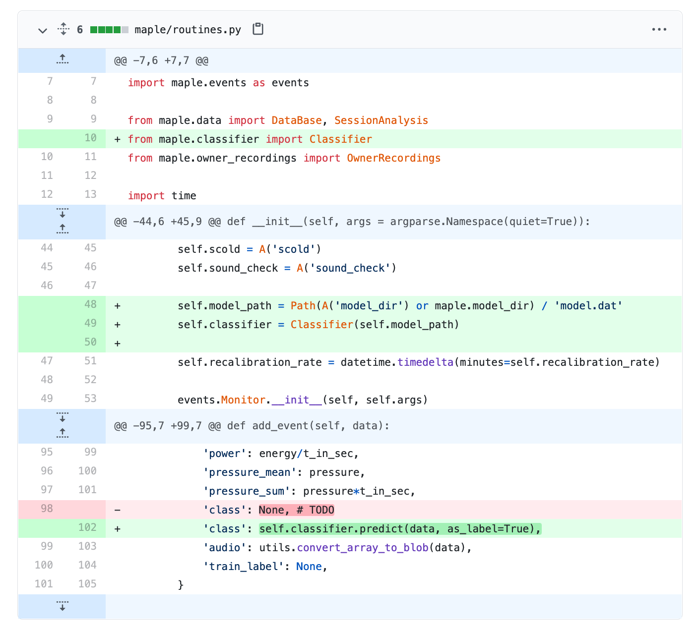
To classify events from past sessions, I extended the command line utility to include a classify mode which makes use of Classifier. It accepts a model directory as input, and optionally a list of session dbs to run the classifier on. It goes through each event of each session db, classifies the event, and stores the results in the class column of the events table. I ran it on all the session DBs with
./main.py classify --model-dir model
This command provides convenient means to classify or re-classify events with a single command, which is super convenient if one day I train a superior classifier and want to apply it to past datasets.
Verdict: pretty accurate
From the training validation I know the accuracy is around 86%, but I wanted to see the classifier in action.
So I loaded up a session database, which now houses fresh labels for each event
./main.py analyze -s 2021_02_13_19_19_33
and used SessionAnalysis.play_many to start comparing the predictions to the audio. Here is a spattering of what I found that included a diverse range of classes.
It’s clearly working pretty well.
Real-time classification
Now I have a way to classify events from past sessions. But moving forward, I would like to classify events as they occur so that the dog-sitter can make real-time decisions on whether to respond to the dog that are based on the class predictions. With the Classifier class in place, this is all I had to change.
Upon this change, all future audio events will be classified on-the-fly.
Speed
One concern about on-the-fly classification is speed. If classification is too slow, I may have to make some sacrifices. For example, tree traversal would be much faster if I decrease the number of trees in the random forest from 200 down to something more light-weight–say 30.
To measure the classification speed, I borrowed a timing class I had written for anvi’o a few years back and put it in maple.utils.
class TimeCode(object):
    """Time a block of code.

    This context manager times blocks of code.

    Examples
    ========
    >>> import time
    >>> import maple.utils as utils
    >>> # EXAMPLE 1
    >>> with utils.TimeCode() as t:
    >>>     time.sleep(5)
    ✓ Code finished successfully after 05s

    >>> # EXAMPLE 2
    >>> with terminal.TimeCode() as t:
    >>>     time.sleep(5)
    >>>     print(asdf) # undefined variable
    ✖ Code encountered error after 05s

    >>> # EXAMPLE 3
    >>> with terminal.TimeCode(quiet=True) as t:
    >>>     time.sleep(5)
    >>> print(t.time)
    0:00:05.000477
    """

    def __init__(self, quiet=False):
        self.s_msg = '✓ Code finished after'
        self.f_msg = '✖ Code encountered error after'
        self.quiet = quiet


    def __enter__(self):
        self.timer = Timer()
        return self


    def __exit__(self, exception_type, exception_value, traceback):
        self.time = self.timer.timedelta_to_checkpoint(self.timer.timestamp())
        return_code = 0 if exception_type is None else 1

        if not self.quiet:
            if return_code == 0:
                print(f"{self.s_msg} {self.time}")
            else:
                print(f"{self.f_msg} {self.time}")
Then, I wrote a script that loads up the audio events of an example session database, and measures the time it takes to classify each event for the classifier. Since I suspected that the number of trees would have a major influence on speed, I went ahead and did these measurements for a spattering of models generated with different tree counts.
#! /usr/bin/env python
import argparse

from maple.data import SessionAnalysis
from maple.utils import TimeCode
from maple.classifier import Train, Classifier

tree_nums = [10, 20, 40, 80, 160, 320, 640]
timing_df = {n: [] for n in tree_nums}

train = Train(argparse.Namespace(label_data = 'label_data.txt'))
train.prep_data()

session = SessionAnalysis(path='data/sessions/2021_02_13_19_19_33/events.db')

for n in tree_nums:
    # Train a model
    train.model_dir = f"model_n_{n}"
    train.setup_dir()
    train.fit_data(param_grid={'n_estimators': [n]}, cv=2)
    train.save()

    # Load the model
    classifier = Classifier(path=f"model_n_{n}/model.dat")

    for _, event in session.dog.iterrows():
        event_audio = event['audio']

        with TimeCode(quiet=True) as t:
            classifier.predict(event_audio)

        timing_df[n].append(t.time)

train.disconnect_dbs()

import seaborn as sns
import matplotlib.pyplot as plt

timing_df = pd.DataFrame(timing_df).melt(var_name='num trees', value_name='time [s]')
timing_df['time [s]'] = timing_df['time [s]'].dt.total_seconds()
timing_df.\
    groupby('num trees').\
    describe().\
    droplevel(0, axis=1).\
    assign(stderr = lambda x: x['std'] /x['count']**(1/2)).\
    plot(kind="bar", y="mean", yerr="stderr")

plt.title('Time-to-classify dependence on tree number')
plt.xlabel('Number of trees [n]')
plt.ylabel('Time [s]')
plt.tight_layout()
plt.show()
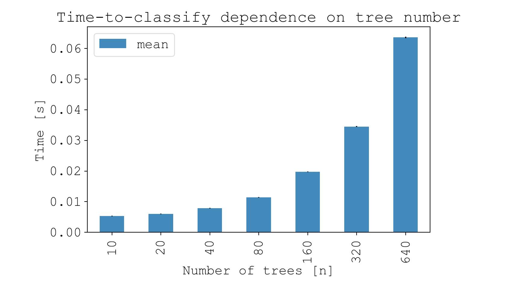
For a model with 200 trees, the cost of classifying during runtime is about 25ms of downtime following each event. Because my application isn’t multi-threaded, this time eats into time that should be dedicated to listening for the next event. Fortunately for me, 25ms is barely anything for my application. On the other hand, a tree count of 640 yields a 60ms downtime, which is starting to become problematic.
Based on these results, I am very happy to keep my model at a tree count of 200.
Section V: Visualizing
One utility of creating an audio classifier is being able to distill the entirety of a session into an intuitive visualization that illustrates how the dogs behaved. Last time I created an interactive interface that can be opened for any session from the command line.
./main.py analyze --session 2021_02_13_19_19_33
Before, it looked like this.
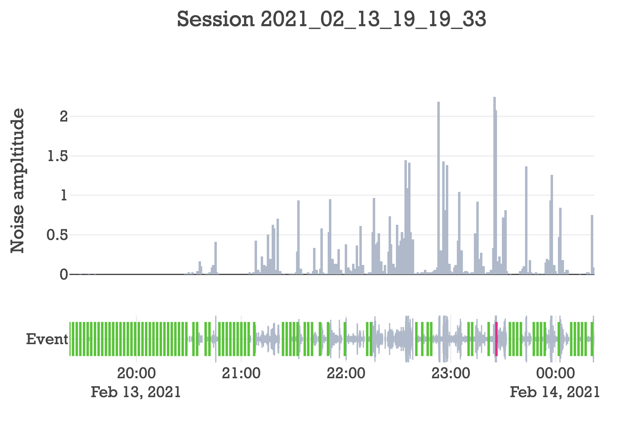
Pretty cool. It shows every event and how loud the dogs were over time. It also shows owner responses, where green is praise and red is scold. But further decomposing the events into their classes would really paint a much more illustrative picture of what’s going on.
I decided that a good way to visualize the data would be to bin the events into minute timeframes and show the proportion of events belonging to each class in a stacked line chart. Ultimately, I decided on the following visual aesthetic:
I create these plots with plotly and the source code can be found here.
With this visualization you can see at a glance how the dog’s behaved. For example, destroying my door seemed to be a passionate side project for Maple, where her progress is apparently driven by repeated bursts of inspiration.
Section VI: Updating response logic
Door scratching is the most undesirable behavior exhibited by the dogs. But in the above session, it went under the radar because it’s not very loud. This is the fundamental problem with the old decision-logic. Yet with real-time classification, now I can buff the decision logic with a more sentiment-based understanding of the events.
The possibilities for buffing the response logic are now endless. I could create different pools of owner responses like praise, scold, warn, console, encourage, etc. But in the interest of me graduating in a timely manner, I decided to keep things pragmatic: I am going to stick to just praise and scold, but I am going to update the decision logic that will take note of the event classes.
Praise
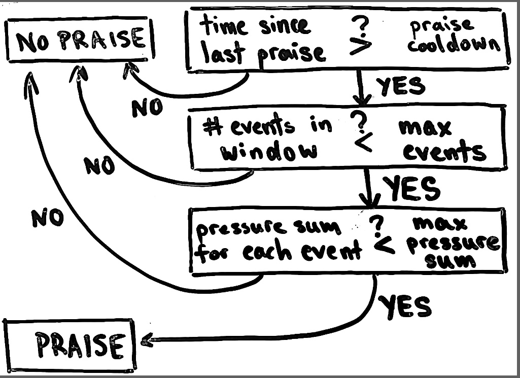
The old logic (above) took note of how many events were in the considered praise window, and enforced (1) that the total number of events should be below some threshold and (2) that none of the events should pass a certain pressure threshold.
This is pretty sound logic, but it fails under circumstances when the dogs produce noise that isn’t inherently bad. Currently, play is the only class that would fall under this category. To accommodate for the fact that noise is not always bad, the new logic is now the same, except all play events in the praise window are removed prior to the logic shown in the above flowchart. This way, the dogs can play and still be praised.
Scold
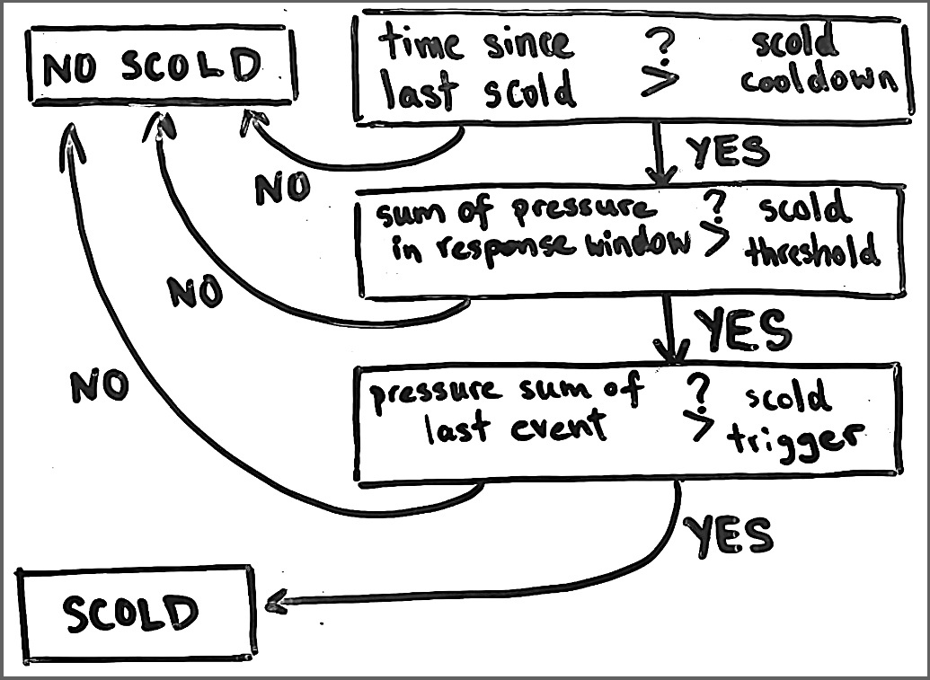
The old logic (above) took note of the total level of noise, whether the most recent event was particularly loud, and if both of these values pass their respective thresholds, the dog-sitter scolds. Again, this is an oversimplification because noise is not always bad.
After re-analyzing sessions, I came to the following new workflow.
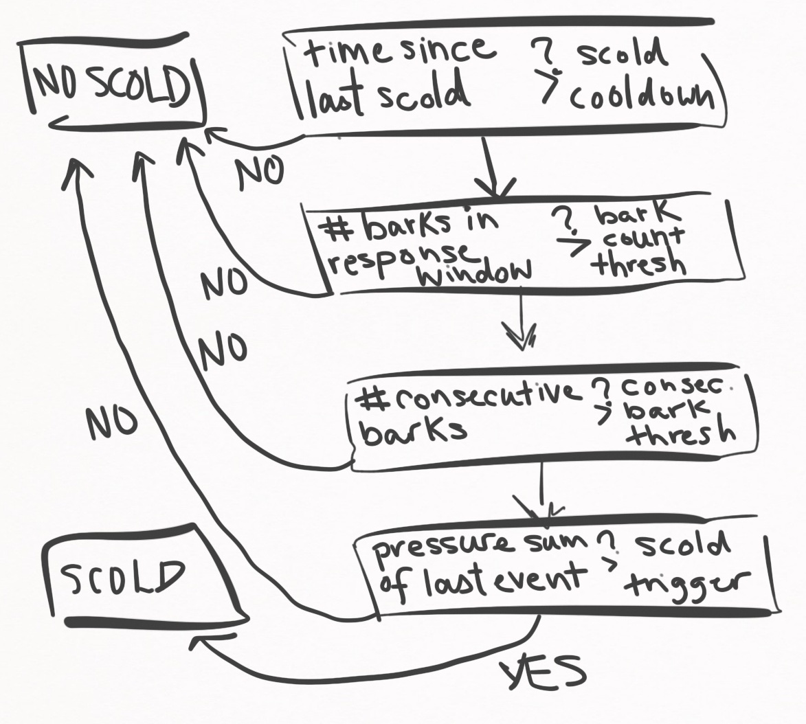
Instead of measuring the total amount of sound pressure, I now count the number of barks. This is first thing that must be triggered to consider a scold. If the number of barks in the scold window is met, then I further demand that that the last $n$ events were all barks. This is just giving them the benefit of the doubt. And then, as a final gift of generosity, I demand that the last event passes some noise threshold. If all these conditions are met, the dog-sitter scolds.
So that’s the workflow for barking. I also wanted to handle door scratching since it is so destructive, so there is another flowchart for scratching.

More simply, the dog-sitter fires off a scold if a certain number of door scratching events are found within the scold window.
Today we’re leaving the house, and these poor doggies are going to be left alone for about 5 hours. A perfect opportunity to test the new decision logic.
Trial run
I nervously set up the system, locked the dogs in the bedroom, and quietly shut the door.
And 5 hours later the results are in. This is a big milestone: first session that implemented real-time audio classification and sentiment-based decision logic.
Considering it was the longest we had left them alone in months, they behaved so well. I’m proud of them. And to be honest, I’m proud of the virtual dog-sitter too, because I think it acted quite rationally.
So I see some door scratching. Were any of the 4 scold responses triggered by door scratching? Here is a zoom-in of the second scold that was properly triggered in response to a series of door scratching events.
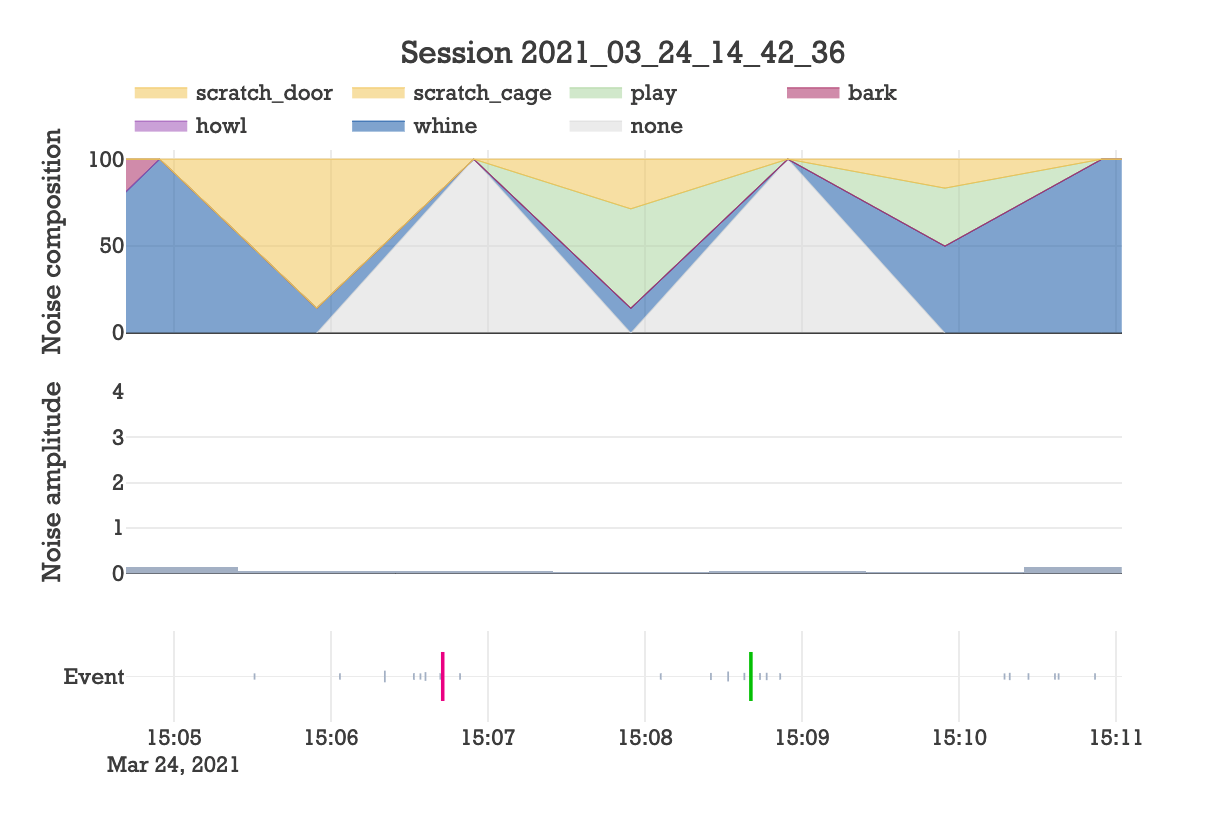
Great! And as cherry on top, the scold seems to have deterred the behavior, at least for a brief minute.
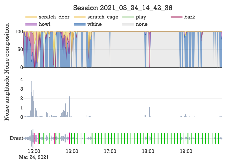
As another example, here is a zoom-in of the first 10 minutes that we were gone, where things got crazy.
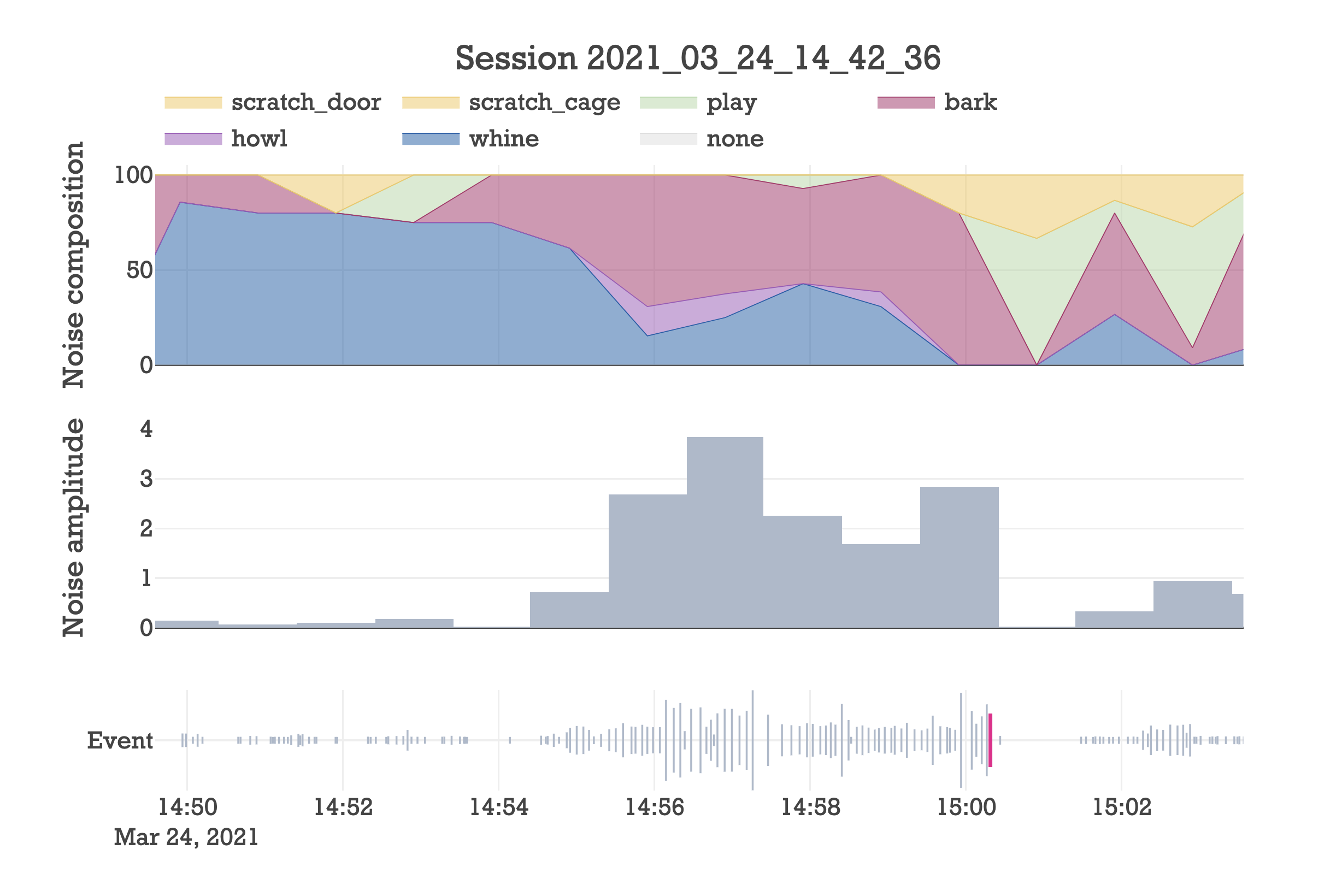
Upon being alone, they are initially struck with worry. Worry that they can’t see their mommy, worry that they heard the front door close, worry that they are no longer in control. This manifests in their vocalizations as whining, and I think it corresponds to them fearing the worst, but trying to keep it together because they want to be good dogs.
Yet as their reality sets in, worry and disbelief turn to panic and desperation. This spiral in mindset is clearly seen as the sound landscape transitions from whining-dominant to barking-dominant. Now unhinged, they continue barking until the dog-sitter decides that enough is enough and scolds them. This seems to snap the dogs back to reality, as evidenced by the abrupt halt in barking.
So the new decision logic for scolding is triggering at the right time, and appears to have a real influence on their behavior.
While the last example shows some very interesting data from a technical standpoint, this is a rather depressing illustration of separation anxiety, something very common in dogs that’s driven by an unhealthy emotional dependence on their owners.
Separation anxiety is essentially the fear of being alone. Currently the dog-sitter addresses separation anxiety by creating the illusion that they are not actually alone. Instead, auditory responses of Kourtney and I give a convincing facade that big brother is watching. This lets them hear our voices and promotes the concept that the same behavorial rules apply even when we are not physically present–which provides them with a sense of normalcy.
So currently separation anxiety is being addressed mostly in an illusory manner. Yet moving forward, I would like the dog-sitter to countercondition the fear associated with being alone, with a newfound excitement of being alone. Currently, all they get for being good is an auditory praise, but what if I created something that dispenses treats instead? A surplus of treats (contingent on good behavior) is certainly a silver lining for being left alone, and would help countercondition a lot of the separation anxiety. If I take this project further, this is the direction I will head.
Conclusion
In summary, this work builds upon the maple software by implementing a random forest classifier that can identify common sounds produced by Maple and Dexter (whine, bark, etc). By classifying events in real time, I was able to develop more robust decisions on how the dog-sitter should respond to the dogs.
All of this new functionality has been implemented in the code base, and the totality of changes made can be viewed in this git compare.
See you next time.
